Support Vector Machines Explained
A Support Vector Machine (SVM) is a very powerful and versatile Machine Learning model, capable of performing linear or nonlinear classification, regression, and even outlier detection. It is one of the most popular models in Machine Learning, and anyone interested in Machine Learning should have it in their toolbox. SVMs are particularly well suited for classification of complex but small- or medium-sized datasets. In this tutorial, I will explain the core concepts of SVMs, how to use them, and how they work.
To explain the SVM, we’ll need to first talk about margins and the idea of separating data with a large “gap”. Next, we’ll talk about the optimal margin classifier. We’ll also see kernels, which give a way to apply SVMs efficiently in very high dimensional (such as infinitedimensional) feature spaces, and finally, we’ll close off the introduction with the SMO algorithm, which gives an efficient implementation of SVMs.
Overview and notation
Previously, we used $\theta$ to parametrizing the hypothesis function $h$. For SVM, we will will use parameters $w$, $b$, and re-write our classifier as:
\[h_{w, b}(x)=g\left(w^{T} x+b\right)\]Where, $g(z) = 1$ if $z \geq 0$, and $g(z) = −1$ otherwise, $b$ takes the role of what was previously $\theta_{0}$ (bias), and $w$ takes the role of $\left[\theta_{1} \ldots \theta_{n}\right]^{T}$ (weights).
Prerequisites
Linearly separable
The first assumption we make so far is that the dataset we have can be linearly seprable.
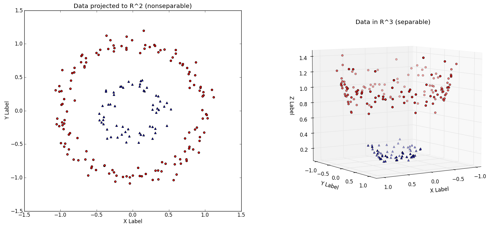
Non-linearly separable and linearly separable. Image resource: Vivek Yadav's Medium blog
The image on the RHS is a case of linearly separable, which is possible to separate the two classes examples by using some separating hyperplane. In this case, Kernel function has been used to project low dimensional data to high dimension. Low dimensional data is not lineary separable, however, it may be linearly separable in a higher dimension.
Lagrange duality
Lagrangian
Optimization problems may be viewed from either of two perspectives, the primal problem or the dual problem.
Consider a optimzation problem as follows:
\[\begin{aligned} {\min_{w}} \quad & {f(w)} \\ \textrm{s.t.} \quad & {h_{i}(w) \quad i=1, \dots, l} \end{aligned}\]Then we define the Lagrangian of the preceding problem as:
\[\mathcal{L}(w, \beta) = f(w) + \sum_{i=1}^{l} \beta_{i} h_{i}(w)\]The $\beta_i$’s are called Lagrange multipliers. The next step is to take the derivatie of $\mathcal{L}$ w.r.t $w$ and $\beta$ and set to zero to solve for $w$ and $\beta$.
Generalized Lagrangian
As we said before, optimization can be viewed as primal problem as well as dual problem. Let us define the primal optimization problem:
\[\begin{aligned} \min_{w} \quad & f(w) \\ \textrm{s.t.} \quad & g_{i}(w) \leq 0, \quad i=1, \dots, k \\ & h_{i}(w)=0, \quad i=1, \dots, l. \end{aligned}\]The generalized Lagrangian is defined as follows:
\[\mathcal{L}(w, \alpha, \beta) = f(w) + \sum \limits_{i=1}^{k} \alpha_i g_i(w) + \sum \limits_{i=1}^{l} \beta_i h_i(w)\]Here, the $\alpha_i$’s and $\beta_i$ ‘s are the Lagrange multipliers.
We use $\mathcal{P}$ to stand for “primal”. If $w$ violates any of the constraints, then we could derive that
\[\begin{aligned} \theta_{\mathcal{P}}(w) &=\max_{\alpha, \beta : \alpha_{i} \geq 0} f(w)+\sum_{i=1}^{k} \alpha_{i} g_{i}(w)+\sum_{i=1}^{l} \beta_{i} h_{i}(w) \\ &=\infty \end{aligned}\]The $\theta_{\mathcal{P}}$ takes the same value as the objective if $w$ satisfies our primal constraints.
\[\min_{w} \theta_{\mathcal{P}}(w) = \min_w \max \limits_{\alpha, \beta: \alpha_i \geq 0} \mathcal{L}(w, \alpha, \beta).\]We use $p^{}$ to stand for the value of the primal problem, which means that $p^{} = \min \limits_{w} \theta_{\mathcal{P}}(w)$. Like we defined $\mathcal{P}$ subscript as primal problem before, we use $\mathcal{D}$ subscript standing for “dual” problem.
\[\max \limits_{\alpha, \beta: \alpha_i \geq 0} \theta_{\mathcal{D}}(\alpha, \beta) = \max \limits_{\alpha, \beta: \alpha_i \geq 0} \min_w \mathcal{L}(w, \alpha, \beta)\]The dual problem and primal problem are related as follows:
\[d^{*} = \max \limits_{\alpha, \beta: \alpha_i \geq 0} \min_w \mathcal{L}(w, \alpha, \beta) \leq \min_w \max \limits_{\alpha, \beta: \alpha_i \geq 0} \mathcal{L}(w, \alpha, \beta) = p^{*}.\]In general, you may think $\max \min \leq \min \max$ is always true.
Under certain conditions, we can get:
\[d^{*} = p^{*}.\]So that we can solver the dual problem in lieu of the primal problem under some conditions.
KKT conditions
Suppose:
- $f$ and the $g_i$’s are convex
- $h_i$’s are affine
- further assumption: $g_i$ are (strictly) feasible
this means that there exists some $w$ so that $g_i(w) < 0$ for all $i$. Under our above assumptions, there must exist $w^{}$ , $\alpha^{}$ , $\beta^{}$ so that $w^{}$ is the solution to the primal problem, $\alpha^{}$ , $\beta^{}$ are the solution to the dual problem, and moreover $p^{} = d^{} = \mathcal{L}(w^{}, \alpha^{}, \beta^{})$. Moreover, $w^{}$ , $\alpha^{}$ , $\beta^{}$ satisfy the Karush-Kuhn-Tucker (KKT) conditions, which are as follows:
\[\begin{aligned} \frac{\partial}{\partial w_{i}} \mathcal{L}\left(w^{*}, \alpha^{*}, \beta^{*}\right) &=0, \quad i=1, \ldots, n \\ \frac{\partial}{\partial \beta_{i}} \mathcal{L}\left(w^{*}, \alpha^{*}, \beta^{*}\right) &=0, \quad i=1, \ldots, l \\ \alpha_{i}^{*} g_{i}\left(w^{*}\right) &=0, \quad i=1, \ldots, k \\ g_{i}\left(w^{*}\right) & \leq 0, \quad i=1, \ldots, k \\ \alpha^{*} & \geq 0, \quad i=1, \ldots, k \end{aligned}\]If some $w^{}$, $\alpha^{}$, $\beta^{*}$ satisfy KKT conditions, then it is also a solution to the primal and dual problems.
KKT dual complementarity condition
\[\alpha_{i}^{*} g_{i}(w^{*}) = 0, \quad i=1, \ldots, k.\]This equation is called KKT dual complementarity condition which is very useful when:
- SVM has only a small number of “support vectors”.
- give convergence test when we talk about the SMO algorithm.
Functional and geometric margins
Functional margin
Consider training example $(x^{(i)}, y^{(i)})$, the functional margin of $(w, b)$ w.r.t. the training example is as follows:
\[\hat{\gamma}^{(i)} = y^{(i)} (w^T x + b).\]A large functional margin represents a confident and a correct prediction. Given training set $S = { (x^{(i)}, y^{(i)}); i = 1,\dots, m }$, we also define the functional margin of $(w, b)$ w.r.t. $S$ to be smallest of the functional margins $\hat{\gamma}$ of the individual training examples.
\[\hat{\gamma} = \min \limits_{i=1, \dots, m} \hat{\gamma}^{(i)}.\]Geometric margin
Let’s now talk ablout geometric margin.
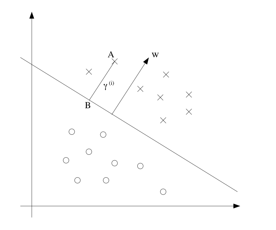
Geometric margin. Image resource: Andrew Ng's lecture notes on SVM
We define geometric margin as:
\[\gamma^{(i)} = y^{(i)} \Large( \large( \frac{w}{\|w\|} \large)^T x^{(i)} + \frac{b}{\|w\|} \Large).\]Given training set $S = { (x^{(i)}, y^{(i)}); i = 1, \dots, m }$, we define the geometric margin of $(w, b)$ w.r.t. $S$ to be smallest of the geometric margins $\gamma$ of the individual training examples.
\[\gamma = \min \limits_{i=1, \dots, m} \gamma^{(i)}.\]Derivation optimal margin classifier
We assume the training set is linearly separable and we would like to find the maximum margin classifier. We pose the following optimization problem:
\[\begin{aligned} \max_{\gamma, w, b} \quad & \gamma \\ \textrm{ s.t. } \quad & y^{(i)}\left(w^{T} x^{(i)}+b\right) \geq \gamma, \quad i=1, \ldots, m \\ &\|w\|=1 \end{aligned}\]$| w | = 1$ ensures that the functional margin equals to geometric margin, but this constraint is “non-convex”. So we transformed this optimization problem as follows:
\[\begin{aligned} \max_{\hat{\gamma}, w, b} \quad & \frac{\hat{\gamma}}{\|w\|} \\ \text { s.t. } \quad & y^{(i)}\left(w^{T} x^{(i)}+b\right) \geq \hat{\gamma}, \quad i=1, \ldots, m \end{aligned}\]Then we scale the factor of $w$ and $b$ to make $\hat{\gamma} = 1$. Note that maximize $\hat{\gamma} / |w| = 1/|w|$ is the same thing as minimize the $|w|^2$. We have the following optimization problem:
\[\begin{aligned} \min_{\gamma, w, b} \quad & \frac{1}{2}\|w\|^{2} \\ \text { s.t. } \quad& y^{(i)}\left(w^{T} x^{(i)}+b\right) \geq 1, \quad i=1, \ldots, m \end{aligned}\]Its solution gives us optimal margin classifier and it is a quadratic programming (QP) problem which can be solved using and QP solver.
Large margin classifiers
According to Largrange duality we re-write the constaints as
\[\begin{aligned} \min_{\gamma, w, b} \quad & \frac{1}{2}\|w\|^{2} \\ \text { s.t. } \quad & 1-y^{(i)} (w^{T} x^{(i)}+b ) \leq 0, \quad i=1, \ldots, m \end{aligned}\]where
\[g_i(w) = 1 - y^{(i)} (w^T x^{(i)} + b) \leq 0\]From KKT dual complementarily condition, we have $\alpha_i > 0$ only for the training examples with contraints $g_i(w) = 0$, where functional margin equals to $1$. The points with the smallest margins are exactly the ones closest to the decision boundary; here, the red points that lie on the dashed lines parallel to the decision boundary. Thus, only two of the $\alpha_i$’s—namely, the ones corresponding to these training examples - will be non-zero at the optimal solution to our optimization problem. These points are called the support vectors in this problem. The fact that the number of support vectors can be much smaller than the size the training set will be useful later.
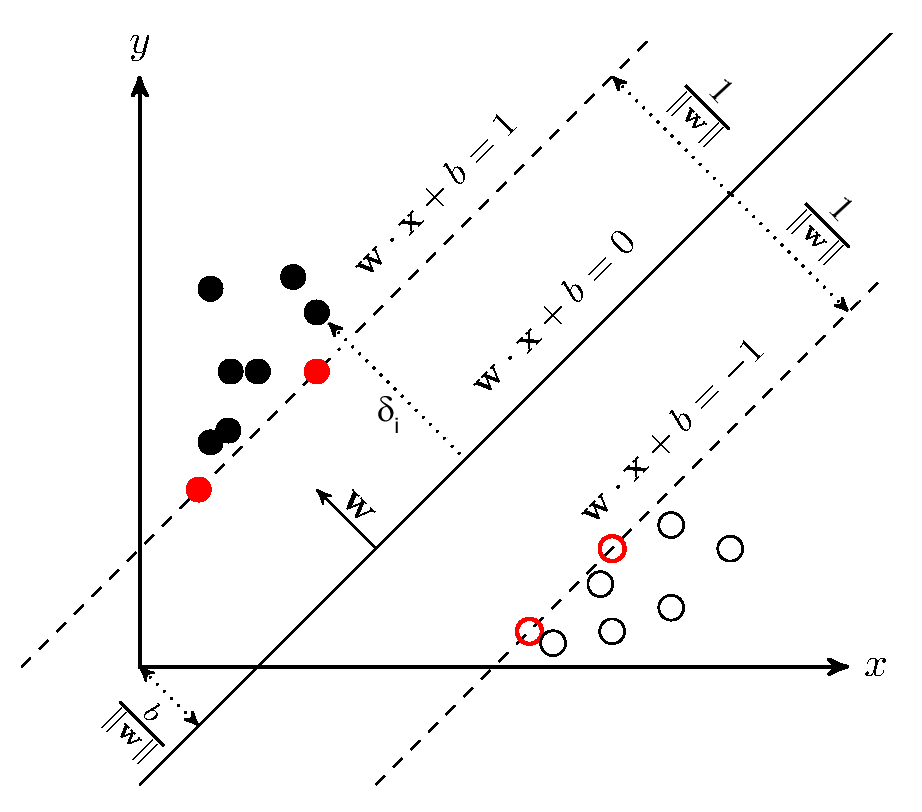
Support Vectors. Image source Michal's blog of "Support vector machines"
Something to remember concerning support vectors:
- functional margin $\hat{\gamma} = 1$
- $\alpha \neq 0$
- $g_i(w) = 0$
Largrangian of optimization problem
The next is to derive Largrangian for the optimization problem we have:
\[\mathcal{L}(w, b, \alpha) = \frac{1}{2} \|w\|^{2} - \sum_{i=1}^{m} \alpha_{i }\left[y^{(i)}\left(w^{T} x^{(i)}+b\right)-1\right].\]Then we need take the derivatives corresponding to $w$ and $\beta$ and we will get:
\[\nabla_{w} \mathcal{L}(w, b, \alpha)=w-\sum_{i=1}^{m} \alpha_{i} y^{(i)} x^{(i)}=0 \Longrightarrow w=\sum_{i=1}^{m} \alpha_{i} y^{(i)} x^{(i)}\]and
\[\frac{\partial}{\partial b} \mathcal{L}(w, b, \alpha)=\sum_{i=1}^{m} \alpha_{i} y^{(i)}=0\]After taking the derivatives corresponding to $w$ and $\beta$, we construct the dual optimization problem:
\[\begin{aligned} \max_{\alpha} \quad & W(\alpha)=\sum_{i=1}^{m} \alpha_{i}-\frac{1}{2} \sum_{i, j=1}^{m} y^{(i)} y^{(j)} \alpha_{i} \alpha_{j}\left\langle x^{(i)}, x^{(j)}\right\rangle \\ \textrm{s.t.} \quad & \alpha_{i} \geq 0, \quad i=1, \ldots, m \\ & \sum_{i=1}^{m} \alpha_{i} y^{(i)}=0 \end{aligned}\]You may be wondering how comes the formula of $W(\alpha)$, you can follow the following steps
\[\begin{aligned} \mathcal{L}(w, b, \alpha) &= \frac{1}{2}\|w\|^{2}-\sum_{i=1}^{m} \alpha_{i}\left[y^{(i)}\left(w^{T} x^{(i)}+b\right)-1\right] \\ &=\frac{1}{2} w^{T} w-\sum_{i=1}^{m} \alpha_{i} y^{(i)} w^{T} x^{(i)}-\sum_{i=1}^{m} \alpha_{i} y^{(i)} b+\sum_{i=1}^{m} \alpha_{i} \\ &=\frac{1}{2} w^{T} \sum_{i=1}^{m} \alpha_{i} y^{(i)} x^{(i)}-\sum_{i=1}^{m} \alpha_{i} y^{(i)} w^{T} x^{(i)}-\sum_{i=1}^{m} \alpha_{i} y^{(i)} b+\sum_{i=1}^{m} \alpha_{i} \\ &=\frac{1}{2} w^{T} \sum_{i=1}^{m} \alpha_{i} y^{(i)} x^{(i)}-w^{T} \sum_{i=1}^{m} \alpha_{i} y^{(i)} x^{(i)}-\sum_{i=1}^{m} \alpha_{i} y^{(i)} b+\sum_{i=1}^{m} \alpha_{i} \\ &=-\frac{1}{2} w^{T} \sum_{i=1}^{m} \alpha_{i} y^{(i)} x^{(i)}-\sum_{i=1}^{m} \alpha_{i} y^{(i)} b+\sum_{i=1}^{m} \alpha_{i} \\ &=-\frac{1}{2} w^{T} \sum_{i=1}^{m} \alpha_{i} y^{(i)} x^{(i)}-b \sum_{i=1}^{m} \alpha_{i} y^{(i)}+\sum_{i=1}^{m} \alpha_{i} \\ &=-\frac{1}{2}\left(\sum_{i=1}^{m} \alpha_{i} y^{(i)} x^{(i)}\right)^{T} \sum_{i=1}^{m} \alpha_{i} y^{(i)} x^{(i)}-b \sum_{i=1}^{m} \alpha_{i} y^{(i)}+\sum_{i=1}^{m} \alpha_{i} \\ &=-\frac{1}{2} \sum_{i=1}^{m} \alpha_{i} y^{(i)}\left(x^{(i)}\right)^{T} \sum_{i=1}^{m} \alpha_{i} y^{(i)} x^{(i)}-b \sum_{i=1}^{m} \alpha_{i} y^{(i)}+\sum_{i=1}^{m} \alpha_{i} \\ &=-\frac{1}{2} \sum_{i, j=1}^{m} \alpha_{i} y^{(i)}\left(x^{(i)}\right)^{T} \alpha_{j} y^{(j)} x^{(j)}-b \sum_{i=1}^{m} \alpha_{i} y^{(i)}+\sum_{i=1}^{m} \alpha_{i} \end{aligned}\]to derive $\mathcal{L}(w, b, \alpha)$, however, in the previous step, we are doing the minimization, so we are maximize the $-\mathcal{L}(w, b, \alpha)$ and we construct the Lagrangian for our optimization problem.
\[\begin{aligned} \mathcal{L}(w, b, \alpha) &=\frac{1}{2} \sum_{i, j=1}^{n} \alpha_{i} \alpha_{j} y_{i} y_{j} x_{i}^{T} x_{j}-\sum_{i, j=1}^{n} \alpha_{i} \alpha_{j} y_{i} y_{j} x_{i}^{T} x_{j}-b \sum_{i=1}^{n} \alpha_{i} y_{i}+\sum_{i=1}^{n} \alpha_{i} \\ &=\sum_{i=1}^{n} \alpha_{i}-\frac{1}{2} \sum_{i, j=1}^{n} \alpha_{i} \alpha_{j} y_{i} y_{j} x_{i}^{T} x_{j} \end{aligned}\]The optimal value for intercept term $b^*$ is:
\[b^{*}=-\frac{\max_{i : y^{(i)}=-1} w^{* T} x^{(i)}+\min _{i : y^{(i)}=1} w^{* T} x^{(i)}}{2}\]Kernels
In the preceding section, we successfully give the optimal value of $w$ in terms of (the optimal value of) $\alpha$. Suppose we’ve fit our model’s parameters to a training set, and now wish to make a prediction at a new point input $x$. We would then calculate $w^T x + b$, and predict $y = 1$ if and only if this quantity is bigger than zero. This quantity can also be written:
\[\begin{aligned} w^{T} x+b &=\left(\sum_{i=1}^{m} \alpha_{i} y^{(i)} x^{(i)}\right)^{T} x+b \\ &=\sum_{i=1}^{m} \alpha_{i} y^{(i)}\left\langle x^{(i)}, x\right\rangle+ b \end{aligned}\]This is very useful as we noticed that there is a inner product part in the formula above. Given a feature mapping $\phi$, we define the kernel $K$ to be defined as:
\[K(x,z)=\phi(x)^T\phi(z)\]We could also define a Kernel matrix $K_{i j}=K\left(x^{(i)}, x^{(j)}\right)$. if $K$ is a valid Kernel, then $K_{i j}=K\left(x^{(i)}, x^{(j)}\right)=\phi\left(x^{(i)}\right)^{T} \phi\left(x^{(j)}\right)=\phi\left(x^{(j)}\right)^{T} \phi\left(x^{(i)}\right)=K\left(x^{(j)}, x^{(i)}\right)=K_{j i}$. Hence $K$ must be symmetric.
Letting $\phi_{k}(x)$ denote the $k$-th coordinate of the vector $\phi(x)$, we find that for any vector $z$, we have
\[\begin{aligned} z^{T} K z &=\sum_{i} \sum_{j} z_{i} K_{i j} z_{j} \\ &=\sum_{i} \sum_{j} z_{i} \phi\left(x^{(i)}\right)^{T} \phi\left(x^{(j)}\right) z_{j} \\ &=\sum_{i} \sum_{j} \sum_{i} \sum_{k} \phi_{k}\left(x^{(i)}\right) \phi_{k}\left(x^{(j)}\right) z_{j} \\ &=\sum_{k} \sum_{i} \sum_{j} z_{i} \phi_{k}\left(x^{(i)}\right) \phi_{k}\left(x^{(j)}\right) z_{j} \\ &=\sum_{k}\left(\sum_{i} z_{i} \phi_{k}\left(x^{(i)}\right)\right)^{2} \\ & \geq 0 \end{aligned}\]Since $z$ was arbitrary, this shows that $K$ is positive semi-definite ($K \geq 0$).
Mercer Theorem
Theorem (Mercer). Let $K : \mathbb{R}^{n} \times \mathbb{R}^{n} \mapsto \mathbb{R}$ be given. Then for $K$ to be a valid (Mercer) kernel, it is necessary and sufficient that for any ${x^{(1)}, \ldots, x^{(m)}}, (m<\infty)$, the corresponding kernel matrix is symmetric positive semi-definite.
Regularization and non-linear separable case
The derivation of the SVM presented so far assumes that the data is linearly separable. Although mapping data to a high-dimensional feature space via $\phi$ usually increases the likelihood of data separability, we cannot guarantee that it will always be. Also, in some cases, it is not clear that finding a separation hyperplane is exactly what we want to do because it can be susceptible to outliers. For example, the left side of the figure below shows an optimal margin classifier. When an outlier is added to the upper left corner (right), it will cause a dramatic swing in the decision boundary, and the resulting classifier is small. The excess amount.
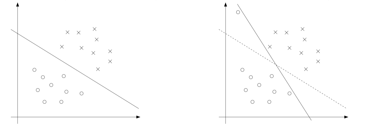
Regularized separating hyperplane in non-linearly separable case.
In order to make SVM work for non-linearly separable datasets as well as less sensitive to outliers. We introduce the $\ell_1$ regularization term, also people call this softmargin SVM.
\[\begin{align*} \min_{r,w,b} \quad & \frac{1}{2}\|w\|^2 + C \sum_{i=1}^{m}{\xi_{i}}\\ \textrm{s.t.} \quad & y^{(i)}(w^T(x^{(i)}+b)) \geq 1 - \xi_{i} \quad i = 1, \dots, m\\ & \xi_i \geq 0 \quad i = 1, \dots, m \\ \end{align*}\]As before, we can form the Lagrangian, and take the derivatives and set to zero:
\[\mathcal{L}(w, b, \xi, \alpha, r)=\frac{1}{2} w^{T} w + C \sum_{i=1}^{m} \xi_{i}-\sum_{i=1}^{m} \alpha_{i}\left[y^{(i)}\left(x^{T} w+b\right)-1+\xi_{i}\right]-\sum_{i=1}^{m} r_{i} \xi_{i}.\]and we can obtain the following dual form of the problem:
\[\begin{aligned} \max_{\alpha} \quad & W(\alpha)=\sum_{i=1}^{m} \alpha_{i}-\frac{1}{2} \sum_{i, j=1}^{m} y^{(i)} y^{(j)} \alpha_{i} \alpha_{j}\left\langle x^{(i)}, x^{(j)}\right\rangle \\ \text { s.t. } \quad & 0 \leq \alpha_{i} \leq C, \quad i=1, \ldots, m \\ & \sum_{i=1}^{m} \alpha_{i} y^{(i)}=0 \end{aligned}\]Also, the KKT dual-complementarity conditions are:
\[\begin{aligned} \alpha_{i}=0 & \Rightarrow y^{(i)}\left(w^{T} x^{(i)}+b\right) \geq 1 \\ \alpha_{i}=C & \Rightarrow y^{(i)}\left(w^{T} x^{(i)}+b\right) \leq 1 \\ 0<\alpha_{i}<C & \Rightarrow y^{(i)}\left(w^{T} x^{(i)}+b\right)=1 \end{aligned}\]Simplified SMO Algorithm
The SMO (sequential mimimal optimization) algorithm gives an efficient way to solve the dual problem arising from the derivation of the SVM problem in a more efficient way. The full SMO algorithm contains many optimizations designed to speed up the algorithm on large datasets and ensure that the algorithm converges even under degenerate conditions.
According to the KKT dual-complementarity conditions in the previous section. Any $\alpha_i$’s that satisfy these properties for all $i$ will be an optimal solution to the optimization problem given above. The SMO algorithm iterates until all these conditions are satisfied (to within a certain tolerance) thereby ensuring convergence.
SMO algorithm could be viewed as the following three steps:
- selects two $\alpha$ parameters, $\alpha_i$ and $\alpha_j$;
- optimizes the objective value jointly for both these $\alpha$’s;
- adjusts the $b$ parameter based on the new $\alpha$’s;
This process is repeated until the $\alpha$’s converge.
Selecting $\alpha$ Parameters
For the simplified version of SMO, we employ a much simple heuristic. We simply iterate over all $\alpha_i, i = 1, \ldots, m$. If $alpha_i$ does not fulfill the KKT conditions to within some numerical tolerance, we select $\alpha_j$ at random from the remaining $m − 1$ $\alpha$’s and attempt to jointly optimize $\alpha_i$ and $\alpha_j$. If none of the $\alpha$s are changed after a few iteration over all the $\alpha_i$’s, then the algorithm terminates.
It is important to realize that by employing this simplification, the algorithm is no longer guaranteed to converge to the global optimum , since we are not attempting to optimize all possible $\alpha_i$, $\alpha_j$ pairs, there exists the possibility that some pair could be optimized which we do not consider.
Optimizing $\alpha_i$ and $\alpha_j$
After choosing the Lagrange multipliers $\alpha_i$ and $\alpha_j$ to optimize, we first compute constraints on the values of these parameters, then we solve the constrained maximization problem.
First we want to find bounds $L$ and $H$ such that $L \leq \alpha_j \leq H$ must hold in order for $\alpha_j$ to satisfy the constraint that $0 \leq \alpha_j \leq C$. It can be shown that these are given by the following:
\[\begin{array}{ll}{\bullet} & {\text { If } y^{(i)} \neq y^{(j)}, \quad L=\max \left(0, \alpha_{j}-\alpha_{i}\right), \quad H=\min \left(C, C+\alpha_{j}-\alpha_{i}\right)} \\ {\bullet} & {\text { If } y^{(i)}=y^{(j)}, \quad L=\max \left(0, \alpha_{i}+\alpha_{j}-C\right), \quad H=\min \left(C, \alpha_{i}+\alpha_{j}\right)}\end{array}\]Now we want to find $\alpha_j$ so as to maximize the objective function. If this value ends up lying outside the bounds $L$ and $H$, we simply clip the value of $\alpha_j$ to lie within this range.
\[\alpha_{j} :=\alpha_{j}-\frac{y^{(j)}\left(E_{i}-E_{j}\right)}{\eta}\]where
\[\begin{aligned} E_{k} &=f\left(x^{(k)}\right)-y^{(k)} \\ \eta &=2\left\langle x^{(i)}, x^{(j)}\right\rangle-\left\langle x^{(i)}, x^{(i)}\right\rangle-\left\langle x^{(j)}, x^{(j)}\right\rangle \end{aligned}\]$E_{k}$ could be treated as the error between the SVM output on the kth example and the true label $y^{(k)}$. Then we used the $\alpha_j$ to find $\alpha_i$
\[\alpha_{i} :=\alpha_{i}+y^{(i)} y^{(j)}\left(\alpha_{j}^{(\mathrm{old})}-\alpha_{j}\right)\]Computing the $b$ threshold
After optimizing $\alpha_i$ and $\alpha_j$ , we select the threshold $b$ such that the KKT conditions are satisfied for the $i$th and $j$th examples. If, after optimization, $\alpha_i$ is not at the bounds (i.e., $0 < \alpha_i < C$), then the following threshold $b_{1}$ is valid, since it forces the SVM to output $y^{(i)}$ when the input is $x^{(i)}$
\[b_{1}=b-E_{i}-y^{(i)}\left(\alpha_{i}-\alpha_{i}^{(\text { old })}\right)\left\langle x^{(i)}, x^{(i)}\right\rangle- y^{(j)}\left(\alpha_{j}-\alpha_{j}^{(\text { old })}\right)\left\langle x^{(i)}, x^{(j)}\right\rangle\]Similarly, the following threshold $b_{2}$ is valid if $0 < \alpha_j < C$
\[b_{2}=b-E_{j}-y^{(i)}\left(\alpha_{i}-\alpha_{i}^{(\text { old })}\right)\left\langle x^{(i)}, x^{(j)}\right\rangle- y^{(j)}\left(\alpha_{j}-\alpha_{j}^{(\text { old })}\right)\left\langle x^{(j)}, x^{(j)}\right\rangle\]If both $0 < \alpha_i < C$ and $0 < \alpha_j < C$ then both these thresholds are valid, and they will be equal. If both new $\alpha$’s are at the bounds (i.e., $\alpha_i = 0$ or $\alpha_i = C$ and $\alpha_j = 0$ or $\alpha_j = C$) then all the thresholds between $b_{1}$ and $b_{2}$ satisfy the KKT conditions, we we let $b := (b1 + b2)/2$. This gives the complete equation for $b$,
\[b :=\left\{\begin{array}{ll}{b_{1}} & {\text { if } 0<\alpha_{i}<C} \\ {b_{2}} & {\text { if } 0<\alpha_{j}<C} \\ {\left(b_{1}+b_{2}\right) / 2} & {\text { otherwise }}\end{array}\right.\]Maximum margin solution in non-linearly separable case
Original form
\[\begin{aligned} \min_{r,w,b} \quad & \frac{1}{2}\|w\|^2 + C \sum_{i=1}^{m}{\xi_{i}} \\ \text{s.t.} \quad & 1- \xi_{i} = y^{(i)}w^Tx^{(i)} \quad i = 1, \ldots, m \\ \end{aligned}\]Regularized form
\[\begin{aligned} \min_{r,w,b} \quad & \sum_{i=1}^{m}{\xi_{i}} + \frac{\lambda}{2}\|w\|^2 \\ \text{s.t.} \quad & 1- \xi_{i} = y^{(i)}w^Tx^{(i)} \quad i = 1, \ldots, m \\ \end{aligned}\]Unconstrained form
\[\begin{aligned} \min_{r,w,b} \quad & \ell_{hinge} (y^{(i)}w^Tx^{(i)}) + \frac{\lambda}{2}\|w\|^2 \\ \text{where} \quad & \ell_{hinge}(z) = \max \{ 0, 1-z \} \\ \end{aligned}\]Hinge loss ― The hinge loss is used in the setting of SVMs and is defined as follows:
\[L(z,y)=[1-yz]_+=\max(0,1-yz)\]Interview Questions
Parameter $C$ in softmargin SVM
Recall the softmargin SVM is as follows:
\[\begin{align*} \min_{r,w,b} \quad & \frac{1}{2}\|w\|^2 + C \sum_{i=1}^{m}{\xi_{i}}\\ \textrm{s.t.} \quad & y^{(i)}(w^T(x^{(i)}+b)) \geq 1 - \xi_{i} \quad i = 1, \dots, m\\ & \xi_i \geq 0 \quad i = 1, \dots, m \\ \end{align*}\]The parameter $C$ tells the algorithm how much you want to avoid mis-classifying each training example.
- For large value of $C$, optimization will choose a smaller-margin hyperplane.
- For small value of $C$, optimization will look for a larger-margin separating hyperplane.
- For tiny value of $C$, will find mis-classified examples, even if data is linearly separable.
Bias-Variance tradeoff of SVMs
We can derive a regularized form of SVM
\[\min_{r,w,b} \quad \frac{1}{2}\|w\|^2 + C \sum_{i=1}^{m}{\xi_{i}}\]to
\[\min_{r,w,b} \quad \sum_{i=1}^{m}{\xi_{i}} + \frac{\lambda}{2}\|w\|^2\]where $\lambda = \frac{1}{C}$.
The paramter $C$ controls the relative weighting between the twin goals of
- making the $|w|^2$ small which makes the margin large.
- ensuring that most examples have functional margin at least $1$.
The procedure of bias-variance tradeoff analysis can be as follows:
- When $C$ is large, which means $\lambda$ is small. We ignore / take away regularization term and lead to a high variance model (overfitting related), so the separating hyperplane is more variable and the margin should be really small.
- When $C$ is small, which mean $\lambda$ is large. We take too much regularization term into account, so that we have a high bias model (underfitting related), so the hyperplane is to ensure the margin is large enough.
Main advantages and drawbacks of SVM
Main advantages
- Mathematically designed to reduce the overfitting by maximizing the margin between data points
- Prediction is fast
- Can manage a lot of data and a lot of features (high dimensional problems)
- Doesn’t take too much memory to store
Main drawbacks
- Can be time consuming to train
- Parameterization can be tricky in some cases
- Communicating isn’t easy
References
- [1] Andrew Ng, CS229: Machine Learning lecture notes, Stanford.
- [2] A. G. Schwing, M. Telgarsky, CS446: Machine Learning lecture slides, UIUC.
- [3] Afshine Amidi and Shervine Amidi, VIP cheatsheets for Stanford’s CS 229 Machine Learning
- [4] Chih-Wei Hsu, Chih-Chung Chang and Chih-Jen Lin, A Practical Guide to Support Vector Classification
- [5] Stack Exachange, When using SVMs, why do I need to scale the features?
- [6] Jose De Dona, Lagrangian Duality
- [7] Stanford CS229, Autumn 2009, The Simplified SMO Algorithm