Week 1 lecture notes: Convolutional Neural Networks
Edge Detection
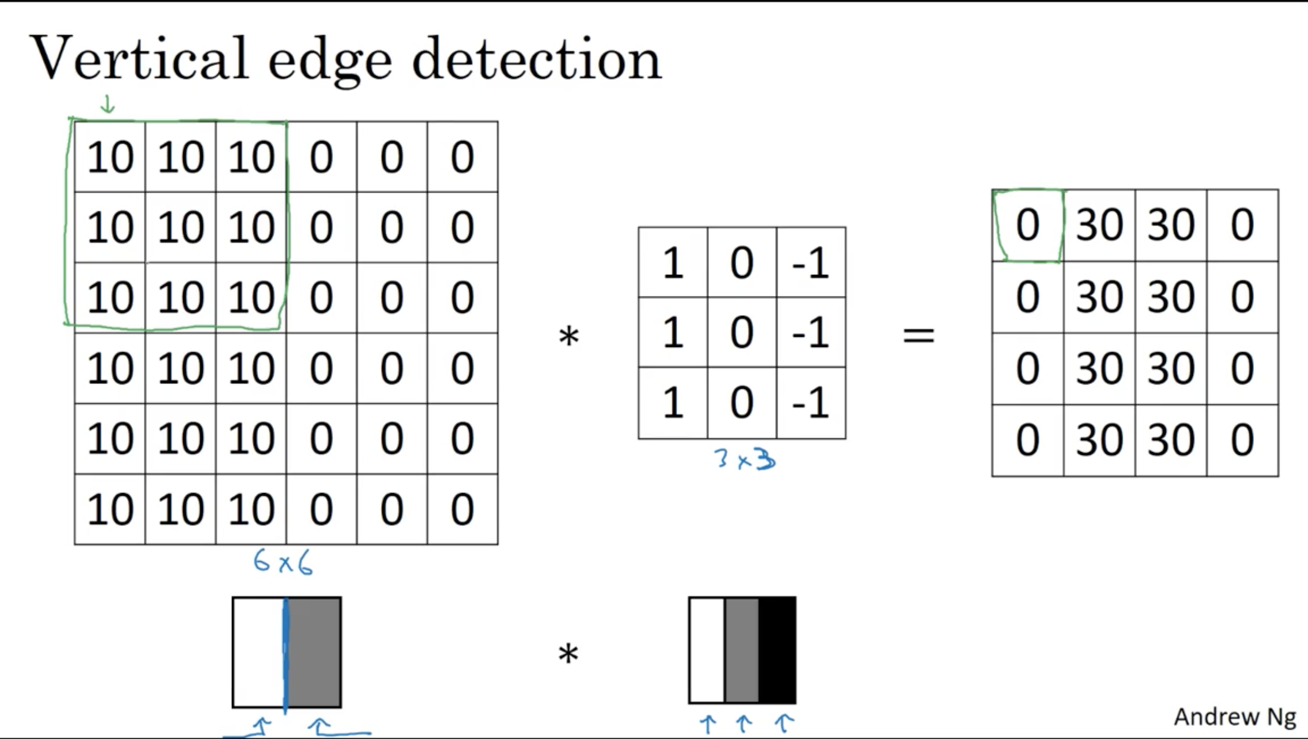
Given an gray-scale image:
\[\begin{bmatrix} 3 & 0 & 1 & 2 & 7 & 4 \\ 1 & 5 & 8 & 9 & 3 & 1 \\ 2 & 7 & 2 & 5 & 1 & 3 \\ 0 & 1 & 3 & 1 & 7 & 8 \\ 4 & 2 & 1 & 6 & 2 & 8 \\ 2 & 4 & 5 & 2 & 3 & 9 \\ \end{bmatrix}\]and a filter (or called kernel):
\[\begin{bmatrix} 1 & 0 & -1 \\ 1 & 0 & -1 \\ 1 & 0 & -1 \end{bmatrix}\]we define convolution $(*)$ operation like image below
After perform convolution, we will get a result:
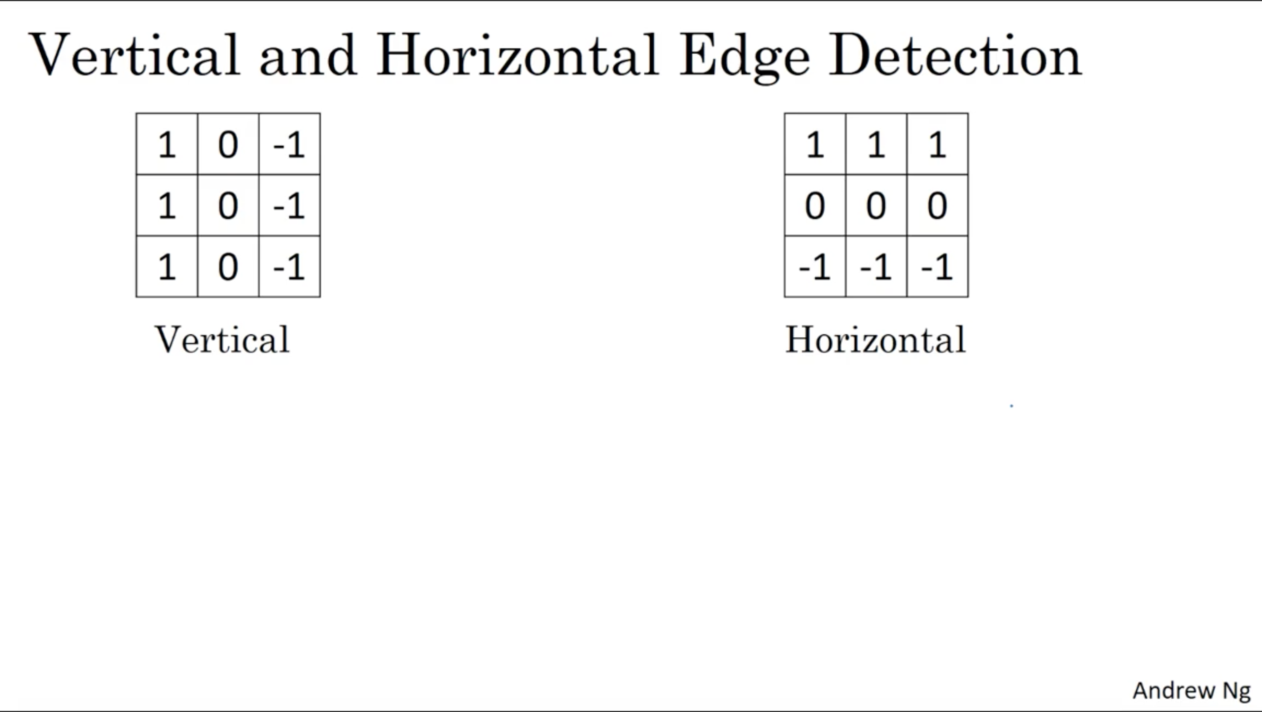
\[\begin{bmatrix} -5 & -4 & 0 & 8 \\ -10 & -2 & 2 & 3 \\ 0 & -2 & -4 & -7 \\ -3 & -2 & -3 & -16 \\ \end{bmatrix}\]Vertical Edge Detection
Horizontal Edge Detection
Sobel operator
\[G_x = \begin{bmatrix} 1 & 0 & -1 \\ 2 & 0 & -2 \\ 1 & 0 & -1 \end{bmatrix} * A\]and
\[G_y = \begin{bmatrix} 1 & 2 & 1 \\ 0 & 0 & 0 \\ -1 & -2 & -1 \end{bmatrix} * A\]where $*$ here denotes the 2-dimensional signal processing convolution operation.
The advantage of using Sobel operator is that it puts more weights to central row and it make the result more robust.
Scharr filter
\[G_x = \begin{bmatrix} 3 & 0 & -3 \\ 10 & 0 & -10 \\ 3 & 0 & -3 \end{bmatrix} * A\]and
\[G_y = \begin{bmatrix} 3 & 10 & 3 \\ 0 & 0 & 0 \\ -3 & -10 & -3 \end{bmatrix} * A\]Learning to detect edges
We could treat the filter as our learning paramters to let the algorithm (back propagation) find the “edge detection” filter or other filters performed on original image.
\[\begin{bmatrix} w_1 & w_2 & w_3 \\ w_4 & w_5 & w_6 \\ w_7 & w_8 & w_9 \end{bmatrix}\]Padding
Padding
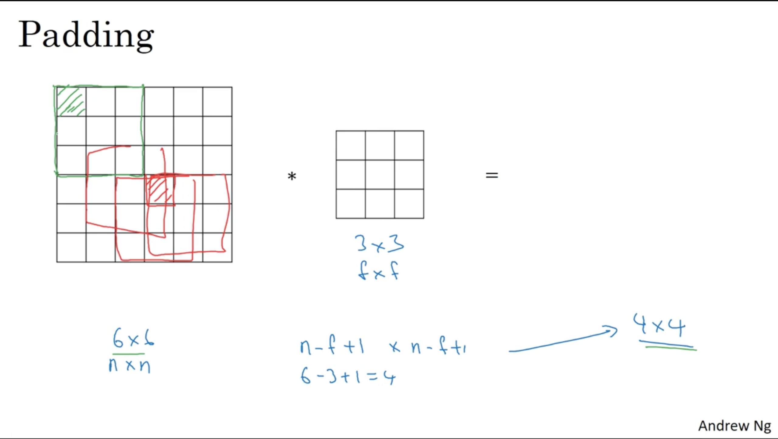
When we perform convolution on the oringinal image:
the green pixel was only used once, however, the red pixel was used much more frequently than the green pixel at the corner. It means that we are throwing much information near the edge of the image and shrinking the output image

Valid and Same convolutions
- Valid: no padding
- Same: Pad so that output image has the same shape as input image \(\begin{align} n + 2p -f + 1 &= n \\ p &= \frac{f - 1}{2} \end{align}\)
$f$ (kernel size / filter size) is usally odd.
Strided convolution
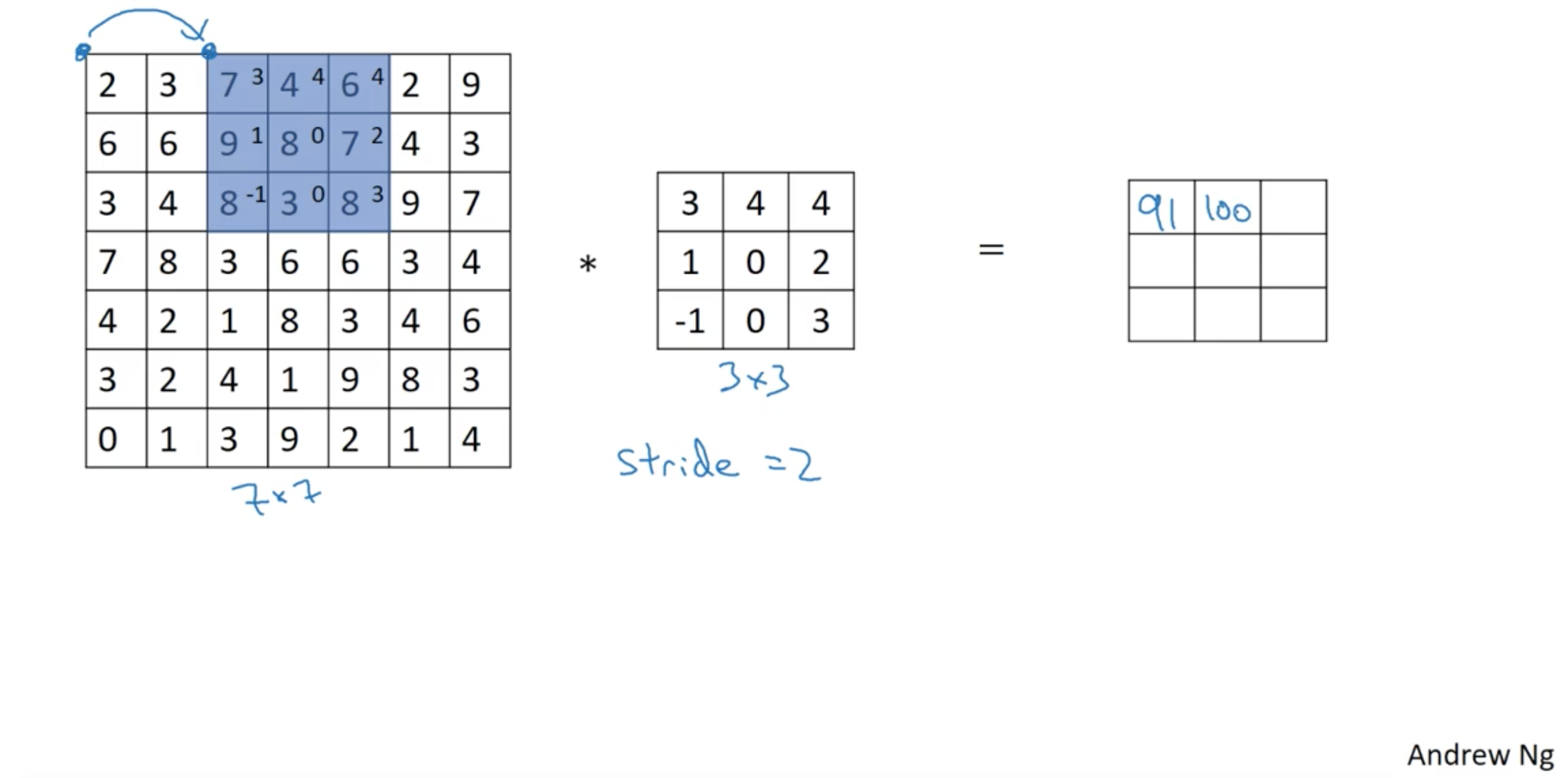
Denote stride using $s$, then result of image with size $n \times n$ with convolution using filter size $f$, padding $p$:
\[\Bigl\lfloor \frac{n + 2p -f}{s} + 1 \Bigr\rfloor \times \Bigl\lfloor \frac{n + 2p -f}{s} + 1 \Bigr\rfloor\]Summary of Convolutions
No padding or strides
The height $d^l_y$ and width $d^l_x$ of the feature maps in the $l$-th layer depend upon the height $d^{l-1}_y$ and width $d^{l-1}_x$ of the feature maps in the previous layer and the size of the filters $ k^l_y \times k^l_x $:
\[\begin{align} d^l_y &= d^{l-1}_y - k^l_y + 1 \\ d^l_x &= d^{l-1}_x - k^l_x + 1 \end{align}\]Padding without strides
Expand the matrices $H_{:,:,p}^{l−1}$ by adding $P$ zeros on all sides to form a larger tensor
\[\hat{H}^{l-1} \in \mathbb{R}^{(d^{l-1}_y + 2P) \times (d^{l-1}_x + 2P) \times C^{l-1}}.\] \[H_{i,j,p}^{l} = \sigma \Bigg( \sum \limits_{p'=0}^{C^{l - 1} - 1} \sum \limits_{m=0}^{k^{l}_{y} - 1} \sum \limits_{n=0}^{k^{l}_{x} - 1} K_{m,n,p,p'}^l H_{i+m,j+n,p'}^{l - 1} \Bigg).\]$H^l$ therefore has dimensions
\[(d^{l-1}_y - k^l_y + 2P + 1) \times (d^{l-1}_x - k^l_x + 2P + 1).\]Strides without padding
A convolution layer with a stride $s$ is
\[H_{i,j,p}^{l} = \sigma \Bigg( \sum \limits_{p'=0}^{C^{l - 1} - 1} \sum \limits_{m=0}^{k^{l}_{y} - 1} \sum \limits_{n=0}^{k^{l}_{x} - 1} K_{m,n,p,p'}^l H_{is+m,js+n,p'}^{l - 1} \Bigg).\]$H^l$ therefore has dimensions
\[\bigg( \Bigl\lfloor \frac{d^{l-1}_y - k_y^l}{s} + 1 \Bigr\rfloor \bigg) \times \bigg( \Bigl\lfloor \frac{d^{l-1}_x - k_x^l}{s} + 1 \Bigr\rfloor \bigg) \times C^l.\]where $C$ stands for channels.
Padding and strides
Expand the matrices $H_{:,:,p}^{l−1}$ by adding $P$ zeros on all sides to form a larger tensor
\[\hat{H}^{l-1} \in \mathbb{R}^{(d^{l-1}_y + 2P) \times (d^{l-1}_x + 2P) \times C^{l-1}}.\]then,
\[H_{i,j,p}^{l} = \sigma \Bigg( \sum \limits_{p'=0}^{C^{l - 1} - 1} \sum \limits_{m=0}^{k^{l}_{y} - 1} \sum \limits_{n=0}^{k^{l}_{x} - 1} K_{m,n,p,p'}^l \hat{H}_{is+m,js+n,p'}^{l - 1} \Bigg).\]$H^l$ therefore has dimensions
\[\bigg( \Bigl\lfloor \frac{d^{l-1}_y - k_y^l + 2P}{s} + 1 \Bigr\rfloor \bigg) \times \bigg( \Bigl\lfloor \frac{d^{l-1}_x - k_x^l + 2P}{s} + 1 \Bigr\rfloor \bigg) \times C^l.\]Convolution over volume
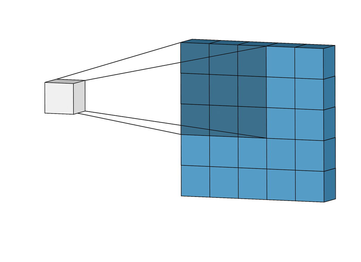
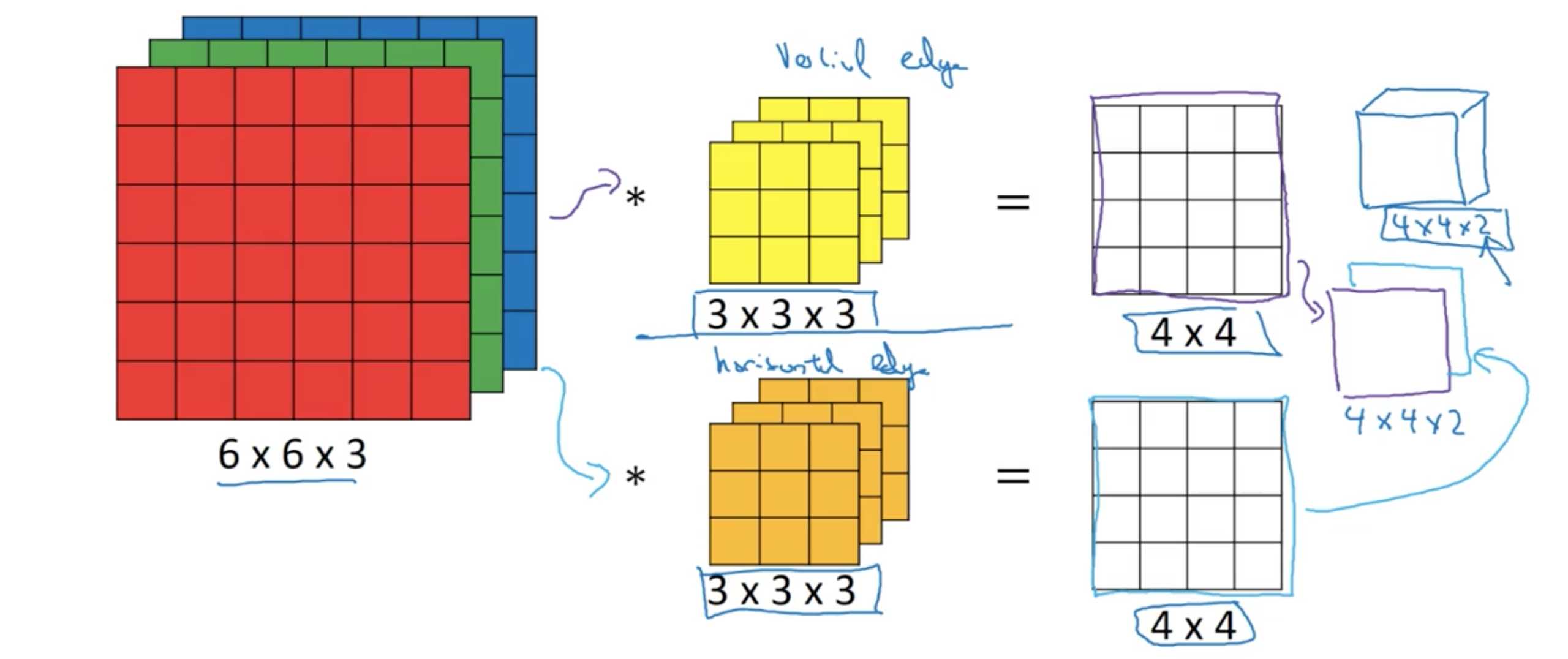
Convolution on RGB image
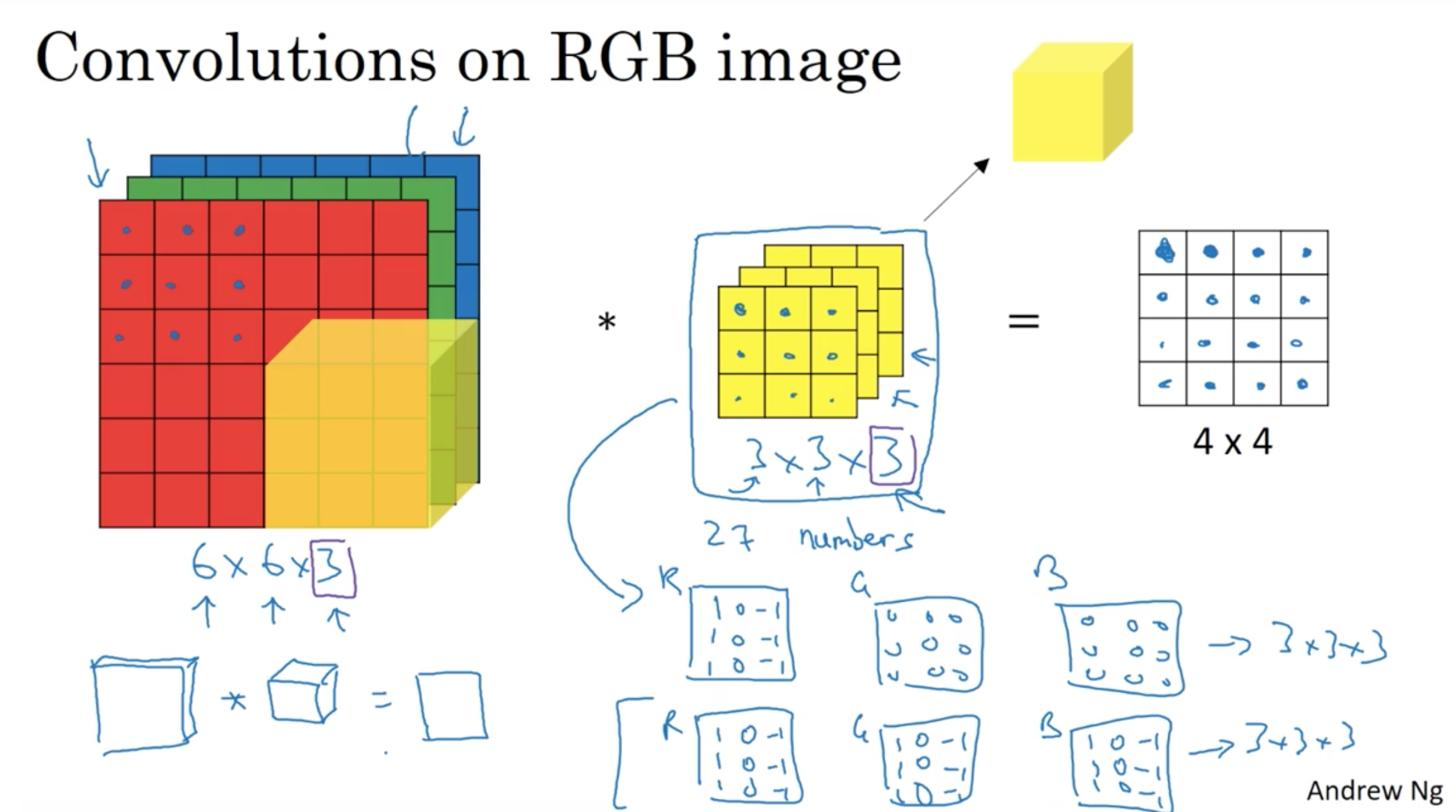
6x6x3 image convolve with 3x3x3 filter giving 4x4x1 output.
Multiple filters
Pooling Layer
It is common to periodically insert a Pooling layer in-between successive Conv layers in a ConvNet architecture. Its function is to progressively reduce the spatial size of the representation to reduce the amount of parameters and computation in the network, and hence to also control overfitting. The Pooling Layer operates independently on every depth slice of the input and resizes it spatially, using the $\max$ operation. The most common form is a pooling layer with filters of size $2 \times 2$ applied with a stride of $2$ downsamples every depth slice in the input by $2$ along both width and height, discarding $75\%$ of the activations. Every $\max$ operation would in this case be taking a max over $4$ numbers (little $2 \times 2$ region in some depth slice). The depth dimension remains unchanged. More generally, the pooling layer:
- Accepts a volume of size $W_1 \times H_1 \times D_1$
- Requires two hyperparameters:
- their spatial extent $F$,
- the stride $S$,
- Produces a volume of size $W_2 \times H_2 \times D_2$ where:
- $ W_2 = (W_1−F)/S+1 $
- $ H_2 = (H_1−F)/S+1 $
- $ D_2 = D_1 $
- Requires two hyperparameters:
- Introduces zero parameters since it computes a fixed function of the input
- For Pooling layers, it is not common to pad the input using zero-padding.
It is worth noting that there are only two commonly seen variations of the max pooling layer found in practice: A pooling layer with $ F=3, S=2 $ (also called overlapping pooling), and more commonly $ F=2, S=2 $. Pooling sizes with larger receptive fields are too destructive.
General pooling. In addition to max pooling, the pooling units can also perform other functions, such as average pooling or even L2-norm pooling. Average pooling was often used historically but has recently fallen out of favor compared to the max pooling operation, which has been shown to work better in practice.
Why convolutions?
- Parameter sharing: A feature detector (such as vertical edge detector) that is useful in one part of the image is probably useful in another part of the image.
- Sparsity of connections: In each layer, each output value depends only on a small number of inputs.
References
[1] Stanford CS231n: Convolutional Neural Networks for Visual Recognition, lecture notes on Convolutional Layer
[2] Stanford CS231n: Convolutional Neural Networks for Visual Recognition, lecture notes on Pooling Layer