Week 2 lecture note of Coursera - Convolutional Neural Networks from deeplearning.ai

Deep convolutional models: case studies

Week 2 lecture notes

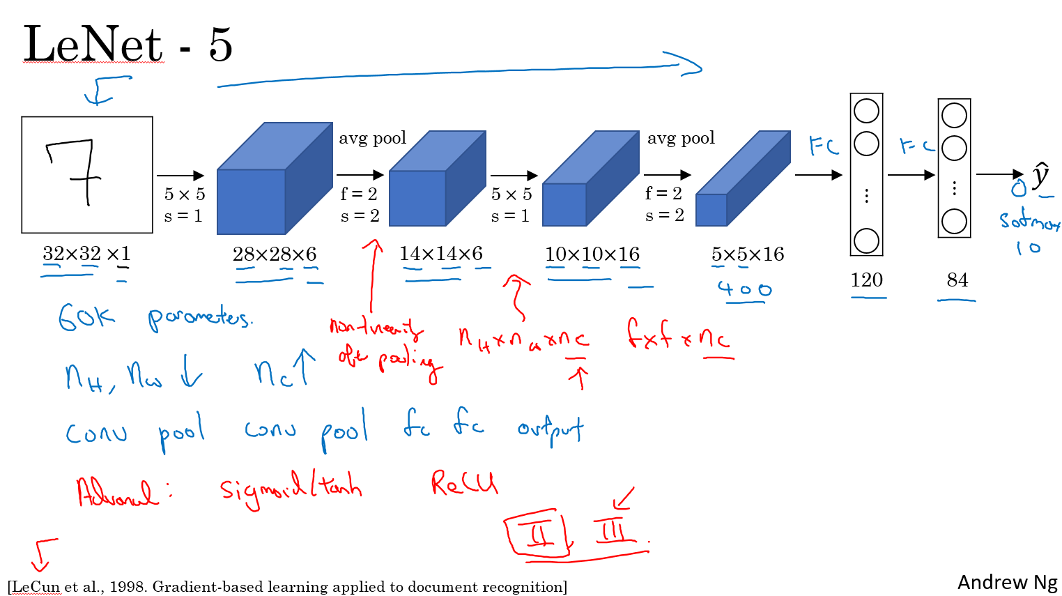
LeNet. The first successful applications of Convolutional Networks were developed by Yann LeCun in 1990’s. Of these, the best known is the LeNet architecture that was used to read zip codes, digits, etc.

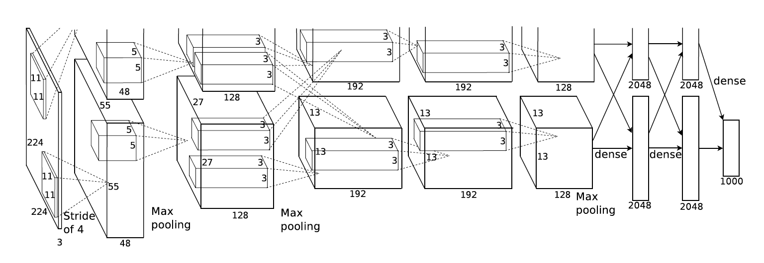
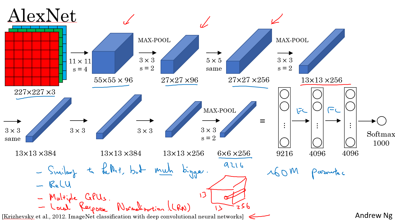
AlexNet. The first work that popularized Convolutional Networks in Computer Vision was the AlexNet, developed by Alex Krizhevsky, Ilya Sutskever and Geoff Hinton. The AlexNet was submitted to the ImageNet ILSVRC challenge in 2012 and significantly outperformed the second runner-up (top 5 error of 16% compared to runner-up with 26% error). The Network had a very similar architecture to LeNet, but was deeper, bigger, and featured Convolutional Layers stacked on top of each other (previously it was common to only have a single CONV layer always immediately followed by a POOL layer).

ZF Net. The ILSVRC 2013 winner was a Convolutional Network from Matthew Zeiler and Rob Fergus. It became known as the ZFNet (short for Zeiler & Fergus Net). It was an improvement on AlexNet by tweaking the architecture hyperparameters, in particular by expanding the size of the middle convolutional layers and making the stride and filter size on the first layer smaller.

GoogLeNet. The ILSVRC 2014 winner was a Convolutional Network from Szegedy et al. from Google. Its main contribution was the development of an Inception Module that dramatically reduced the number of parameters in the network (4M, compared to AlexNet with 60M). Additionally, this paper uses Average Pooling instead of Fully Connected layers at the top of the ConvNet, eliminating a large amount of parameters that do not seem to matter much. There are also several followup versions to the GoogLeNet, most recently Inception-v4.

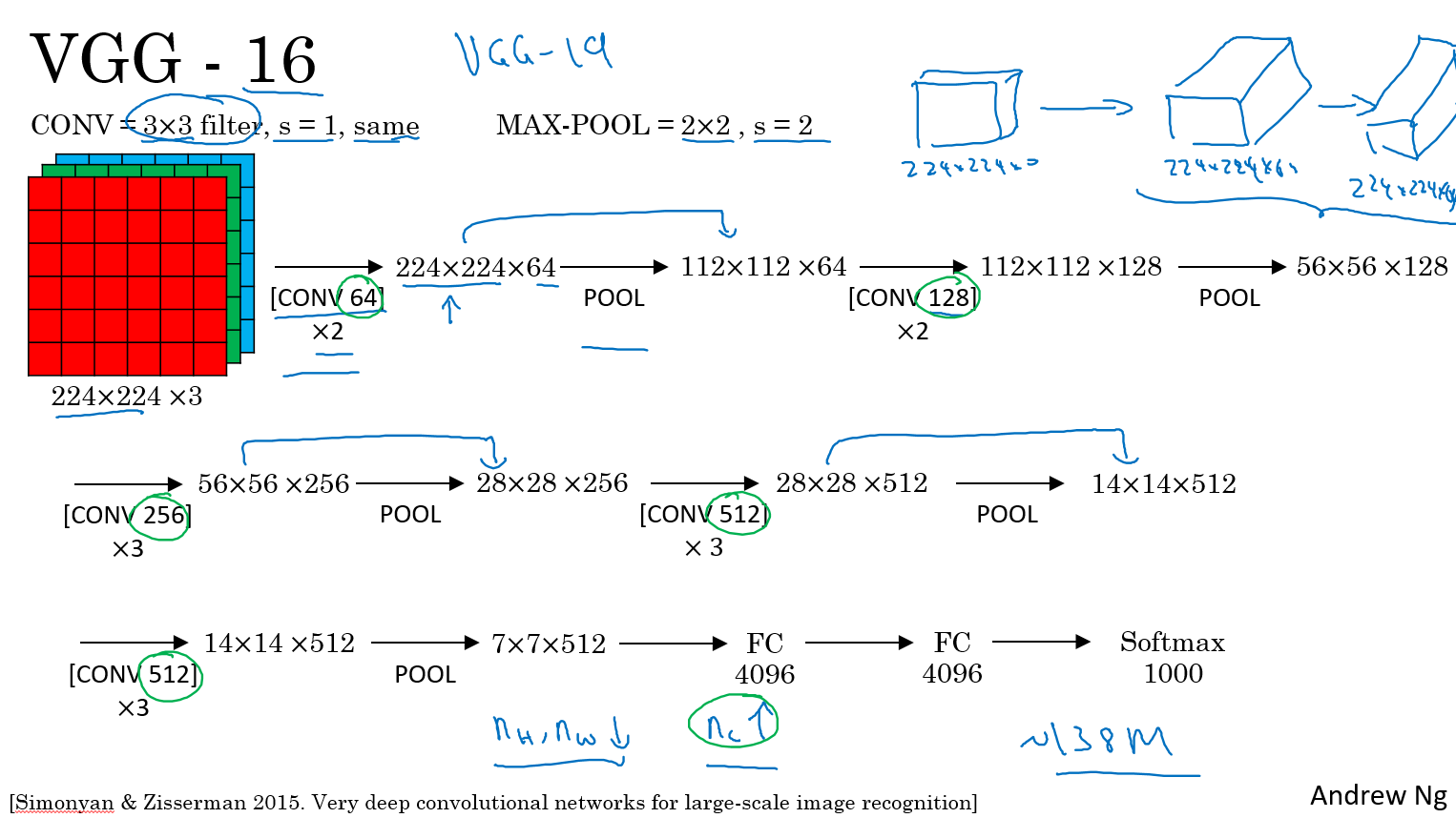
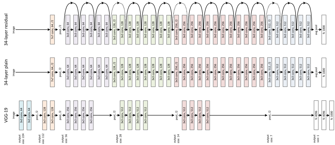
VGGNet. The runner-up in ILSVRC 2014 was the network from Karen Simonyan and Andrew Zisserman that became known as the VGGNet. Its main contribution was in showing that the depth of the network is a critical component for good performance. Their final best network contains 16 CONV/FC layers and, appealingly, features an extremely homogeneous architecture that only performs 3x3 convolutions and 2x2 pooling from the beginning to the end. Their pretrained model is available for plug and play use in Caffe. A downside of the VGGNet is that it is more expensive to evaluate and uses a lot more memory and parameters (140M). Most of these parameters are in the first fully connected layer, and it was since found that these FC layers can be removed with no performance downgrade, significantly reducing the number of necessary parameters.

ResNet. Residual Network developed by Kaiming He et al. was the winner of ILSVRC 2015. It features special skip connections and a heavy use of batch normalization. The architecture is also missing fully connected layers at the end of the network. The reader is also referred to Kaiming’s presentation (video, slides), and some recent experiments that reproduce these networks in Torch. ResNets are currently by far state of the art Convolutional Neural Network models and are the default choice for using ConvNets in practice (as of May 10, 2016). In particular, also see more recent developments that tweak the original architecture from Kaiming He et al. Identity Mappings in Deep Residual Networks (published March 2016).

LeNet - 5

AlexNet

VGG - 16

ResNet

Residual block

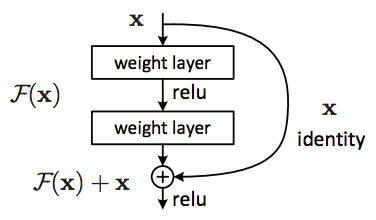
Instead of hoping each stack of layers directly fits a desired underlying mapping, we explicitly let these layers fit a residual mapping. The original mapping is recast into $F(x) + x$. We hypothesize that it is easier to optimize the residual mapping than to optimize the original, unreferenced mapping. To the extreme, if an identity mapping were optimal, it would be easier to push the residual to zero than to fit an identity mapping by a stack of nonlinear layers.

We have reformulated the fundamental building block (figure above) of our network under the assumption that the optimal function a block is trying to model is closer to an identity mapping than to a zero mapping, and that it should be easier to find the perturbations with reference to an identity mapping than to a zero mapping. This simplifies the optimization of our network at almost no cost. Subsequent blocks in our network are thus responsible for fine-tuning the output of a previous block, instead of having to generate the desired output from scratch.

Network in Network (1 by 1 conv)

Most simplistic explanation would be that $1 \times 1$ convolution leads to dimension reductionality. For example, an image of $200 \times 200$ with $50$ features on convolution with $20$ filters of $1 \times 1$ would result in size of $200 \times 200 \times 20$.

Feature transformation

Although $1 \times 1$ convolution is a “feature pooling” technique, there is more to it than just sum pooling of features across various channels/feature-maps of a given layer. $1 \times 1$ convolution acts like coordinate-dependent transformation in the filter space. It is important to note here that this transformation is strictly linear, but in most of application of $1 \times 1$ convolution, it is succeeded by a non-linear activation layer like ReLU. This transformation is learned through the (stochastic) gradient descent. But an important distinction is that it suffers with less over-fitting due to smaller kernel size ($1 \times 1$).

Deeper Network

One by One convolution was first introduced in this paper titled Network in Network. In this paper, the author’s goal was to generate a deeper network without simply stacking more layers. It replaces few filters with a smaller perceptron layer with mixture of $1 \times 1$ and $3 \times 3$ convolutions. In a way, it can be seen as “going wide” instead of “deep”, but it should be noted that in machine learning terminology, “going wide” is often meant as adding more data to the training. Combination of $1 \times 1 (\times F)$ convolution is mathematically equivalent to a multi-layer perceptron.

Inception Network

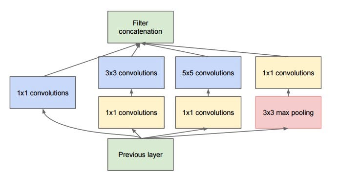
Bottleneck layer

The bottleneck layer of Inception was reducing the number of features, and thus operations, at each layer, so the inference time could be kept low. Before passing data to the expensive convolution modules, the number of features was reduce by, say, $4$ times. This led to large savings in computational cost, and the success of this architecture.

Let’s examine this in detail. Let’s say you have 256 features coming in, and $256$ coming out, and let’s say the Inception layer only performs $3 \times 3$ convolutions. That is $256 \times 256 \times 3 \times 3$ convolutions that have to be performed ($589000$s multiply-accumulate, or MAC operations). That may be more than the computational budget we have, say, to run this layer in 0.5 milli-seconds on a Google Server. Instead of doing this, we decide to reduce the number of features that will have to be convolved, say to $64$ or $256/4$. In this case, we first perform $256 \rightarrow 64 1 \times 1$ convolutions, then $64$ convolution on all Inception branches, and then we use again a $1 \times 1$ convolution from $64 \rightarrow 256$ features back again. The operations are now:

$256 \times 64 \times 1 \times 1 = 16000 \text{s}$
$64 \times 64 \times 3 \times 3 = 36000 \text{s}$
$64 \times 256 \times 1 \times 1 = 16000 \text{s}$

For a total of about $70000$ versus the almost $600000$, almost 10x less operations!

Transfer Learning

For all the examples in training sets, save them to disk and then just train the softmax function right on top of that. The advantage of the safety disk or the pre-compute method or the safety disk is that you don’t need to recompute those activations everytime you take a epoch or take a post through a training set.

If your dataset is larger, one approach is to freeze some layers, that means that freeze the parameters, no updating for those layers’ parameters.

If you have more data, the number of layers to be frozen should be smaller and the number of layers you train on top could be larger.

If you have a lot lot lot of data, then you should use the existed models (pre-trained models) and train on your dataset without freezing layers.

Data Augmentation

Common Data Augmentation

Mirroring
Random cropping
Rotation
Shearing
Local warping
etc..

Color Shifting

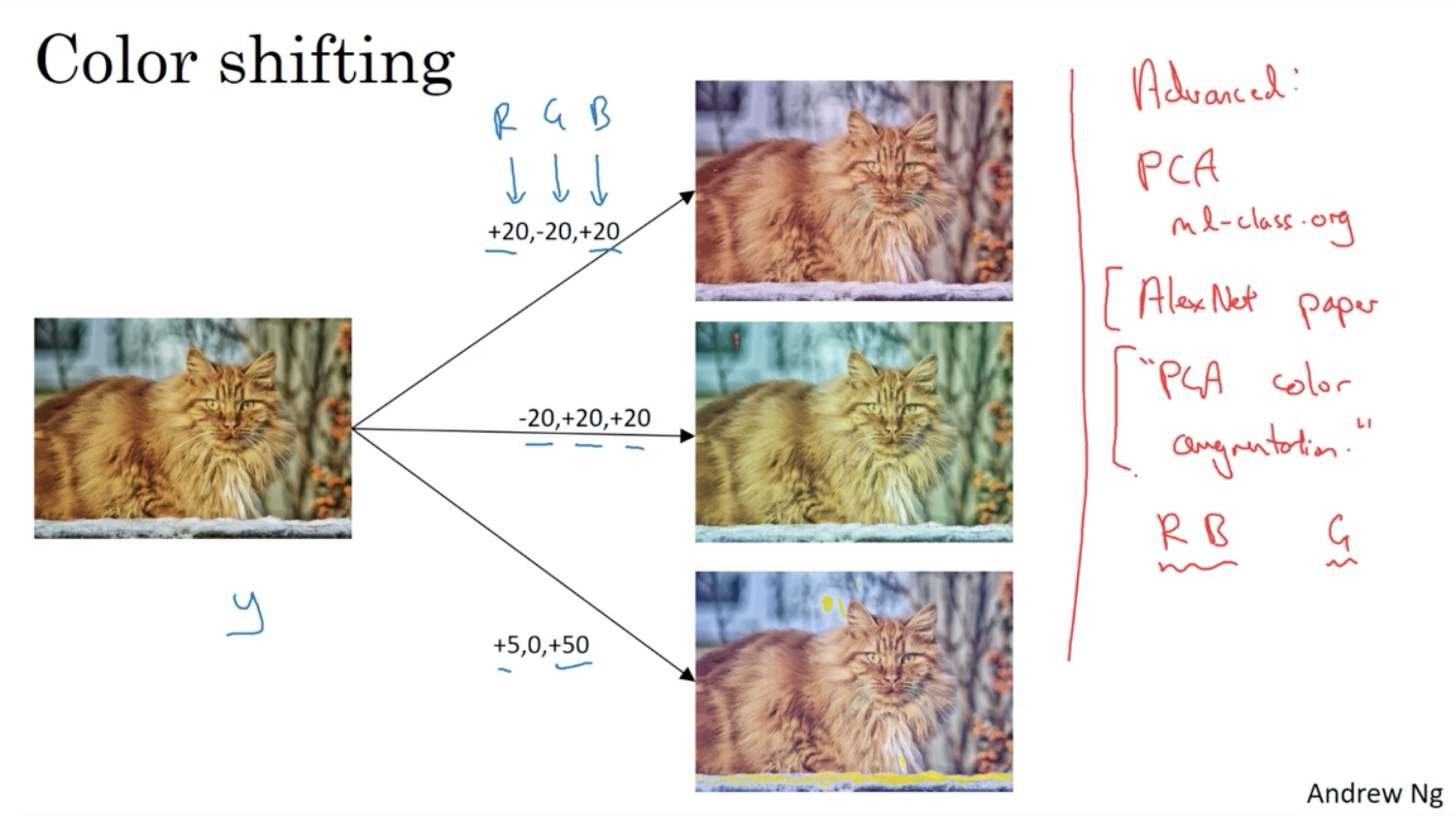
Advanced: PCA color augmentation

For every image each pixel is a data point which is having 3 vectors: R,G,B. You can compute co-variance matrix of these vectors in order to compute the PCA.

If you take 3x3 matrix size, computing PCA results in 3 vectors with 3 components. You can then sample 3 scale parameters, and add scaled versions of each of these 3 vectors to all pixels in the image. For best results you should also scale them by the corresponding eigenvalues. This will perturb the image colors along these PCA axes.

If PCA vectors have larger eigenvalue than the others, so it was clearly dominant and can be equivalent with brightness perturbation instead of color perturbation.