Week 3 lecture note of Coursera - Convolutional Neural Networks from deeplearning.ai

Object detection

Week 3 lecture notes

Object Localization

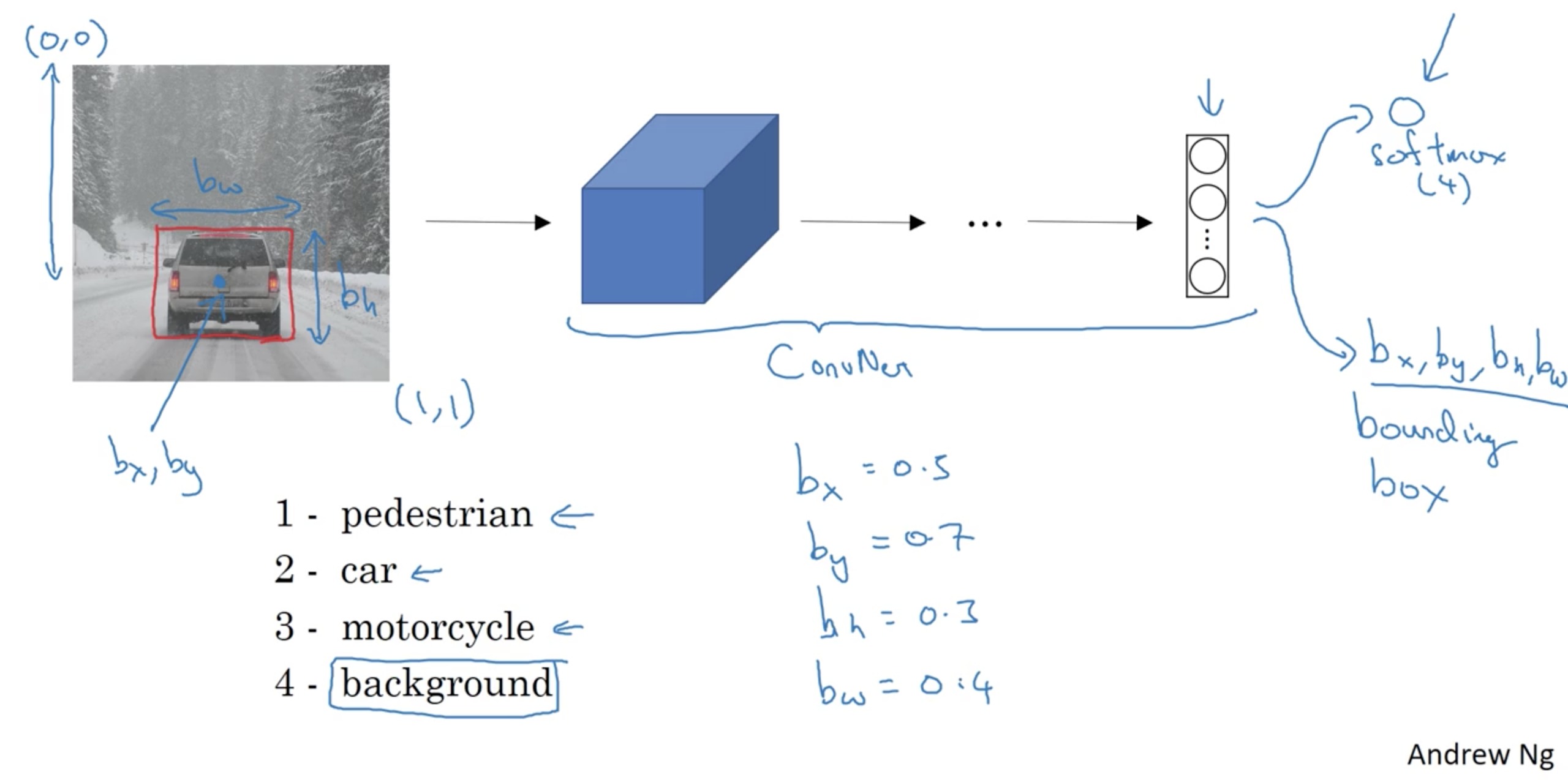
Classification with Localization

Defining the target label y

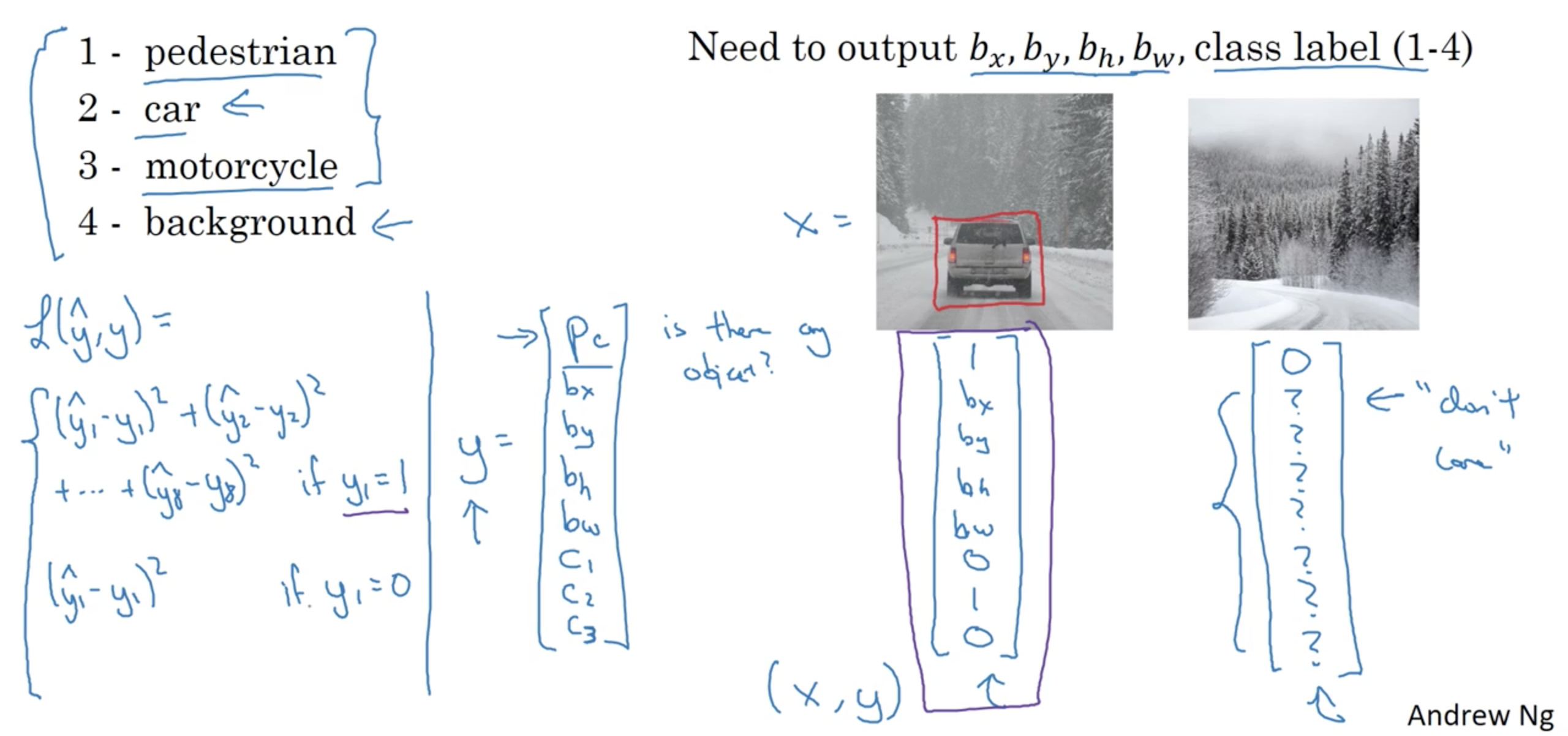
Loss function is defined as follows:

\[\mathcal{L}(\hat{y}, y)= \begin{cases} (\hat{y}_1 - y_1)^2 + (\hat{y}_2 - y_2)^2 + \cdots + (\hat{y}_n - y_n)^2,& \text{if } y_1 = 1\\ (\hat{y}_1 - y_1)^2, & \text{if } y_1 = 0 \end{cases}\]

Landmark Detection

Object Detection

Sliding windows detection

Example of the sliding a window approach, where we slide a window from left-to-right and top-to-bottom.

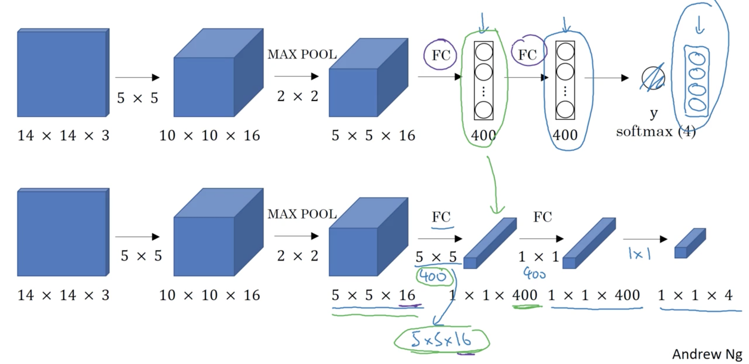
Convolutional Implementation of Sliding Windows

Turning FC layers to Convolutional layers

Bounding Box Predictions

YOLO Algorithm

You only look once (YOLO) is a state-of-the-art, real-time object detection system. On a Pascal Titan X it processes images at 30 FPS and has a mAP of 57.9% on COCO test-dev.

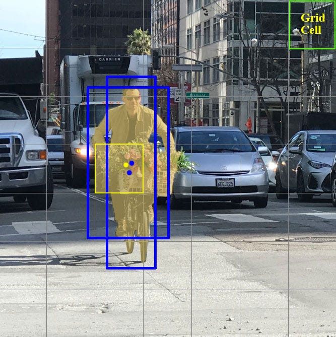
YOLO divides the input image into an $S \times S$ grid. Each grid cell predicts only one object. For example, the yellow grid cell below tries to predict the “person” object whose center (the blue dot) falls inside the grid cell.

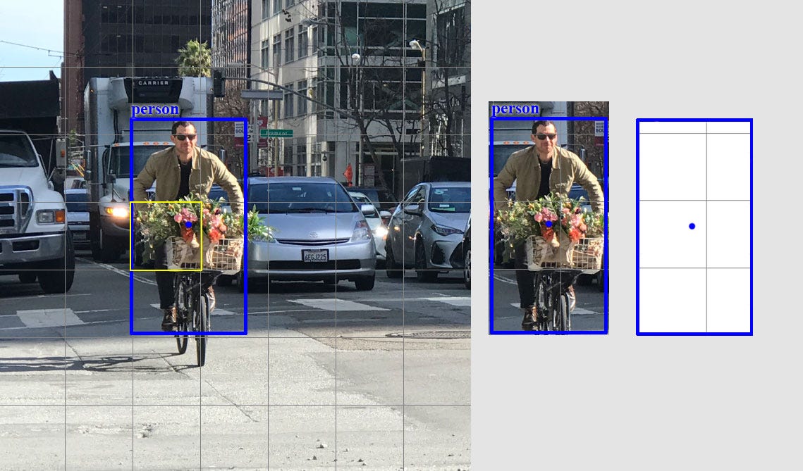
Each grid cell predicts a fixed number of boundary boxes. In this example, the yellow grid cell makes two boundary box predictions (blue boxes) to locate where the person is.

Intersection over Union

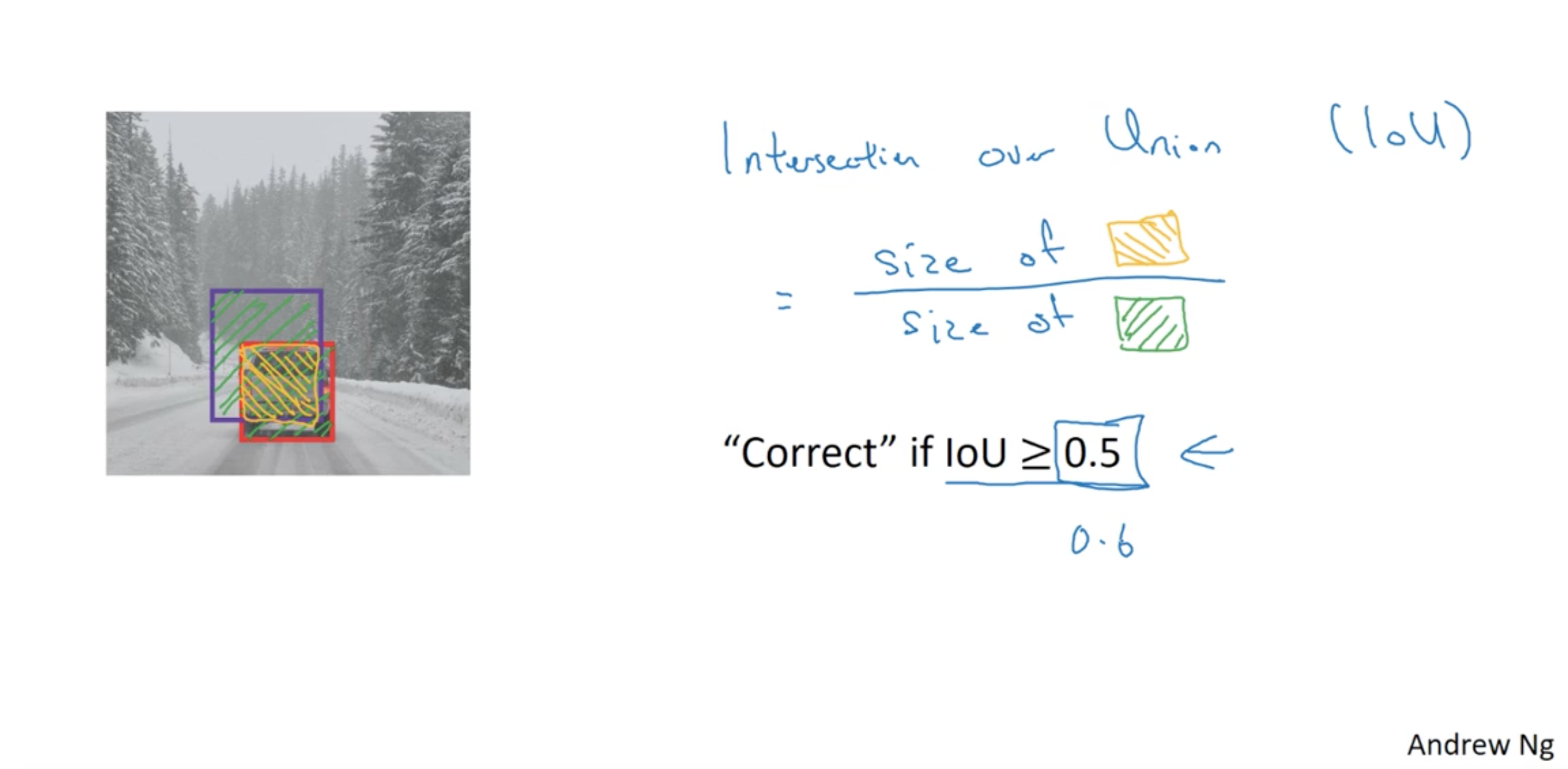
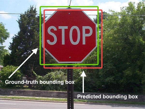
Intersection over Union is an evaluation metric used to measure the accuracy of an object detector on a particular dataset. More formally, in order to apply Intersection over Union to evaluate an (arbitrary) object detector we need:

The ground-truth bounding boxes (i.e., the hand labeled bounding boxes from the testing set that specify where in the image our object is).
The predicted bounding boxes from our model.

Figure 1: Illustration of Intersection over Union. The predicted bounding box is drawn in red while the ground-truth bounding box is drawn in green. Our goal is to compute the Intersection of Union between these bounding box. (Image Source: *Intersection over Union (IoU) for object detection*)

How to compute IoU?

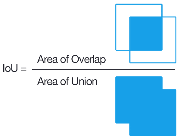
Figure 2: Computing the Intersection of Union is as simple as dividing the area of overlap between the bounding boxes by the area of union. (Image Source: *Intersection over Union (IoU) for object detection*)

In the numerator we compute the area of overlap between the predicted bounding box and the ground-truth bounding box. The denominator is the area of union, or more simply, the area encompassed by both the predicted bounding box and the ground-truth bounding box.

\[\text{IoU} = \frac{\text{Area of Overlap}}{\text{Area of Union}}\]

Non-max Suppression

Python implementation from `Pyimageserach.com`

# import the necessary packages
import numpy as np

#  Felzenszwalb et al.
def non_max_suppression_slow(boxes, overlapThresh):
	# if there are no boxes, return an empty list
	if len(boxes) == 0:
		return []

	# initialize the list of picked indexes
	pick = []

	# grab the coordinates of the bounding boxes
	x1 = boxes[:,0]
	y1 = boxes[:,1]
	x2 = boxes[:,2]
	y2 = boxes[:,3]

	# compute the area of the bounding boxes and sort the bounding
	# boxes by the bottom-right y-coordinate of the bounding box
	area = (x2 - x1 + 1) * (y2 - y1 + 1)
	idxs = np.argsort(y2)

We’ll start on Line 2 by importing a single package, NumPy, which we’ll utilize for numerical processing.

From there we define our non_max_suppression_slow function on Line 5. this function accepts to arguments, the first being our set of bounding boxes in the form of (startX, startY, endX, endY) and the second being our overlap threshold. I’ll discuss the overlap threshold a little later on in this post.

Lines 7 and 8 make a quick check on the bounding boxes. If there are no bounding boxes in the list, simply return an empty list back to the caller.

From there, we initialize our list of picked bounding boxes (i.e. the bounding boxes that we would like to keep, discarding the rest) on Line 11.

Let’s go ahead and unpack the (x, y) coordinates for each corner of the bounding box on Lines 14-17 — this is done using simple NumPy array slicing.

Then we compute the area of each of the bounding boxes on Line 21 using our sliced (x, y) coordinates.

Be sure to pay close attention to Line 22. We apply np.argsort to grab the indexes of the sorted coordinates of the bottom-right y-coordinate of the bounding boxes. It is absolutely critical that we sort according to the bottom-right corner as we’ll need to compute the overlap ratio of other bounding boxes later in this function.

Now, let’s get into the meat of the non-maxima suppression function:

# import the necessary packages
import numpy as np

#  Felzenszwalb et al.
def non_max_suppression_slow(boxes, overlapThresh):
	# if there are no boxes, return an empty list
	if len(boxes) == 0:
		return []

	# initialize the list of picked indexes
	pick = []

	# grab the coordinates of the bounding boxes
	x1 = boxes[:,0]
	y1 = boxes[:,1]
	x2 = boxes[:,2]
	y2 = boxes[:,3]

	# compute the area of the bounding boxes and sort the bounding
	# boxes by the bottom-right y-coordinate of the bounding box
	area = (x2 - x1 + 1) * (y2 - y1 + 1)
	idxs = np.argsort(y2)

	# keep looping while some indexes still remain in the indexes
	# list
	while len(idxs) > 0:
		# grab the last index in the indexes list, add the index
		# value to the list of picked indexes, then initialize
		# the suppression list (i.e. indexes that will be deleted)
		# using the last index
		last = len(idxs) - 1
		i = idxs[last]
		pick.append(i)
		suppress = [last]

We start looping over our indexes on Line 26, where we will keep looping until we run out of indexes to examine.

From there we’ll grab the length of the idx list o Line 31, grab the value of the last entry in the idx list on Line 32, append the index i to our list of bounding boxes to keep on Line 33, and finally initialize our suppress list (the list of boxes we want to ignore) with index of the last entry of the index list on Line 34.

That was a mouthful. And since we’re dealing with indexes into a index list it’s not exactly an easy thing to explain. But definitely pause here and examine these code as it’s important to understand.

Time to compute the overlap ratios and determine which bounding boxes we can ignore:

# import the necessary packages
import numpy as np

#  Felzenszwalb et al.
def non_max_suppression_slow(boxes, overlapThresh):
	# if there are no boxes, return an empty list
	if len(boxes) == 0:
		return []

	# initialize the list of picked indexes
	pick = []

	# grab the coordinates of the bounding boxes
	x1 = boxes[:,0]
	y1 = boxes[:,1]
	x2 = boxes[:,2]
	y2 = boxes[:,3]

	# compute the area of the bounding boxes and sort the bounding
	# boxes by the bottom-right y-coordinate of the bounding box
	area = (x2 - x1 + 1) * (y2 - y1 + 1)
	idxs = np.argsort(y2)

	# keep looping while some indexes still remain in the indexes
	# list
	while len(idxs) > 0:
		# grab the last index in the indexes list, add the index
		# value to the list of picked indexes, then initialize
		# the suppression list (i.e. indexes that will be deleted)
		# using the last index
		last = len(idxs) - 1
		i = idxs[last]
		pick.append(i)
		suppress = [last]

		# loop over all indexes in the indexes list
		for pos in xrange(0, last):
			# grab the current index
			j = idxs[pos]

			# find the largest (x, y) coordinates for the start of
			# the bounding box and the smallest (x, y) coordinates
			# for the end of the bounding box
			xx1 = max(x1[i], x1[j])
			yy1 = max(y1[i], y1[j])
			xx2 = min(x2[i], x2[j])
			yy2 = min(y2[i], y2[j])

			# compute the width and height of the bounding box
			w = max(0, xx2 - xx1 + 1)
			h = max(0, yy2 - yy1 + 1)

			# compute the ratio of overlap between the computed
			# bounding box and the bounding box in the area list
			overlap = float(w * h) / area[j]

			# if there is sufficient overlap, suppress the
			# current bounding box
			if overlap > overlapThresh:
				suppress.append(pos)

		# delete all indexes from the index list that are in the
		# suppression list
		idxs = np.delete(idxs, suppress)

	# return only the bounding boxes that were picked
	return boxes[pick]

Here we start looping over the (remaining) indexes in the idx list on Line 37, grabbing the value of the current index on Line 39.

Using last entry in the idx list from Line 32 and the current entry in the idx list from Line 39, we find the largest (x, y) coordinates for the start bounding box and the smallest (x, y) coordinates for the end of the bounding box on Lines 44-47.

Doing this allows us to find the current smallest region inside the larger bounding boxes (and hence why it’s so important that we initially sort our idx list according to the bottom-right y-coordinate). From there, we compute the width and height of the region on Lines 50 and 51.

So now we are at the point where the overlap threshold comes into play. On Line 55 we compute the overlap , which is a ratio defined by the area of the current smallest region divided by the area of current bounding box, where “current” is defined by the index j on Line 39.

If the overlap ratio is greater than the threshold on Line 59, then we know that the two bounding boxes sufficiently overlap and we can thus suppress the current bounding box. Common values for overlapThresh are normally between 0.3 and 0.5.

Line 64 then deletes the suppressed bounding boxes from the idx list and we continue looping until the idx list is empty.

Finally, we return the set of picked bounding boxes (the ones that were not suppressed) on Line 67.

Anchor Boxes

Anchor Box Algorithm

YOLO Algorithm

YOLO uses a single CNN network for both classification and localising the object using bounding boxes. This is the architecture of YOLO:

In the end, the model will output a tensor with shape of $7 \times 7 \times 30$.

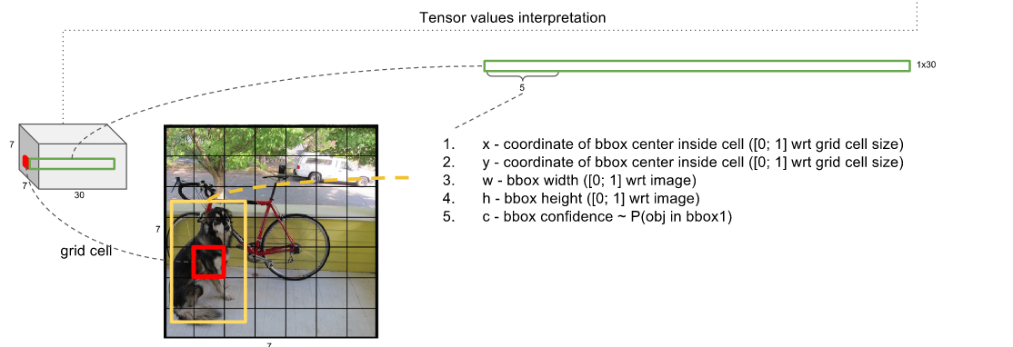
2 Box definitions: (consisting of: $x$, $y$ , width, height,”is object” confidence)
20 class probabilities (only considered if the “is object” confidence is high)

Where:

$S$: Tensor spatial dimension (7 in this case)
$B$: Number of bounding boxes (x, y, w, h, confidence)
$C$: Number of classes
$\text{confidence} = \text{P}_{\text{object}}.\text{IoU}(\text{pred}, \text{gt})$

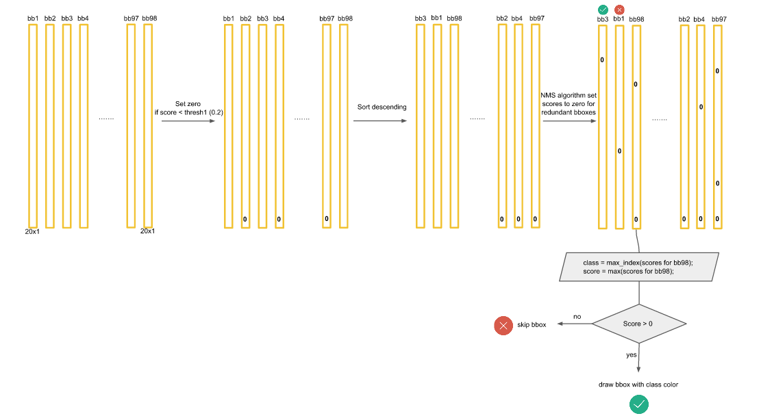
Now we have class scores for each bounding box(Tensor dimension=20*1). Now let us focus on the dog in the image. The dog score for the bounding boxes will be present in (1,1) of the tensor in all the bounding box scores. We will now set a threshold value of scores and sort them descendingly.

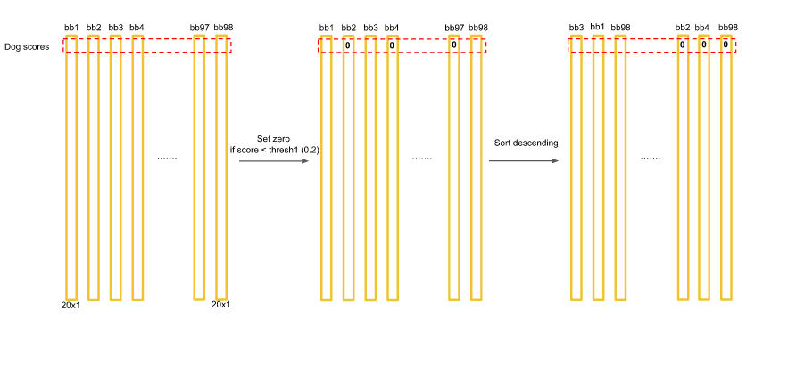
Now we will use Non-max supression algorithm to set score to zero for redundant boxes.

Consider you have dog score for boundingbox1 as 0.5 and let this be the highest score and for box47 as 0.3. We will take an Intersection over Union of these values and if the value is greater than 0.5, we will set the value for box2 as zero,otherwise, we will continue to the next box. We do this for all boxes.

After all this has been done, we will be left with 2–3 boxes only. All others will be zero. Now, we select bbox to draw by class score value. This is explained in the image.