Week 4 lecture note of Coursera - Convolutional Neural Networks from deeplearning.ai

Special applications: Face recognition & Neural style transfer

Week 4 lecture notes

Face verification v.s. Face recognition

Verfication

Input: image, name/ID
Output: Whether the imput image is that of the claimed person

Recognition

Has a database of K persons
Get an input image
Output ID if the image is any of the K persons (or “not recognized”)

One Shot Learning

Learning a “similarity” function

$d(\text{img1}, \text{img2})$ - degree of difference of two images

if $d(\text{img1}, \text{img2}) \leq \tau$, where $\tau$ is a threshold parameter, then predict these two images are “same”

Siamese Network

Siamese networks are a special type of neural network architecture. Instead of a model learning to classify its inputs, the neural networks learns to differentiate between two inputs. It learns the similarity between them.

Parameters of NN define an encoding $f(x^{(i)})$

Learn parameters so that:

If $x^{(i)}, x^{(j)}$ are the same person, $| f(x^{(i)}) - f(x^{(j)})|^2$ is small
If $x^{(i)}, x^{(j)}$ are different person, $| f(x^{(i)}) - f(x^{(j)})|^2$ is large

The architecture

A Siamese networks consists of two identical neural networks, each taking one of the two input images. The last layers of the two networks are then fed to a contrastive loss function , which calculates the similarity between the two images. I have made an illustration to help explain this architecture.

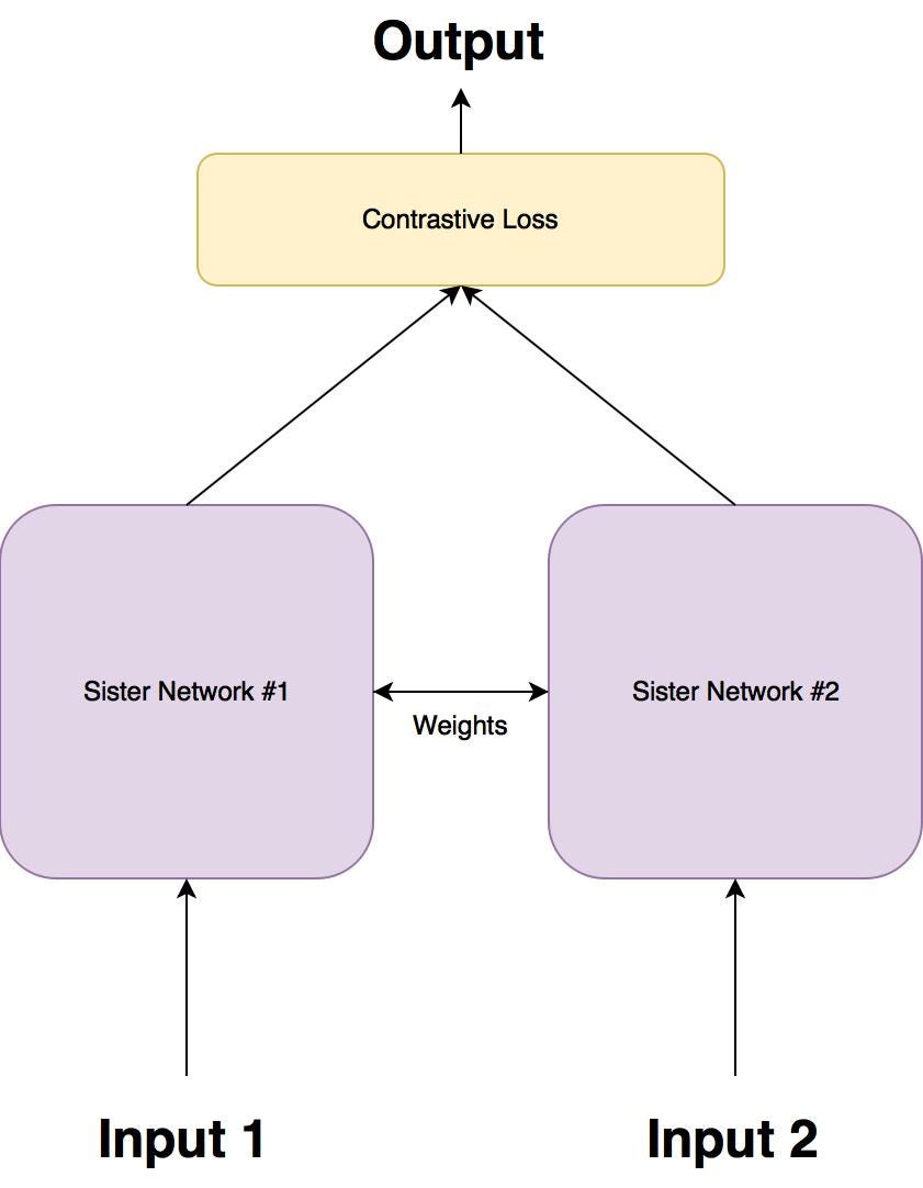
There are two sister networks, which are identical neural networks, with the exact same weights.

Each image in the image pair is fed to one of these networks. The networks are optimised using a contrastive loss function(we will get to the exact function).

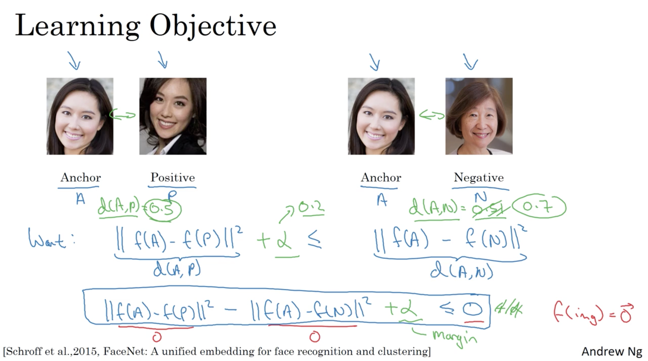
Triplet Loss

Learning objective

Loss function

$p_i$: Input to the $Q$ (Query) network. This image is randomly sampled across any class.
$p_i^+$: Input to the $P$ (Positive) network. This image is randomly sampled from the SAME class as the query image.
$p_i^-$: Input to the $N$ (Negative) network. This image is randomly sample from any class EXCEPT the class of $p_i$.

triplet loss. It teaches the network to produce similar feature embeddings for images from the same class (and different embeddings for images from different classes).

\[l(p_i, p_i^+, p_i^-) = \max \{ 0, g + D \big(f(p_i), f(p_i^+) \big) - D \big( f(p_i), f(p_i^-) \big) \}\]

$D$ is the Euclidean Distance between $f(p_i)$ and $f(p_i^{+/-})$.

\[D(p, q) = \sqrt{(q_1 − p_1)^2 + (q_2 − p_2)^2 + \dots + (q_n − p_n)^2}\]

$g$ is the gap parameter that regularizes the gap between the distance of two image pairs: $(p_i, p_i^+)$ and $(p_i, p_i^-)$.

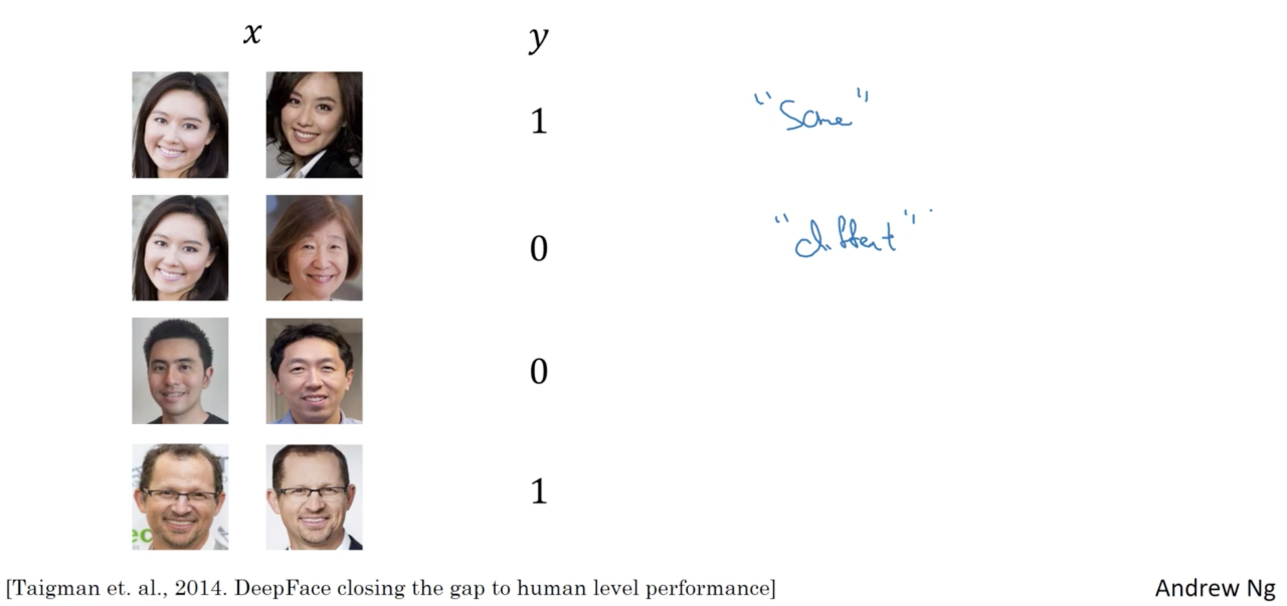
Face Verification and Binary Classification

Neural Style Transfer

Neural style transfer cost function

We use $C$ to denote content image, the image will be “style transfered”, $S$ to denote style image and $G$ to denote generated image

Cost function is defined using a content cost function and style cost function

\[J(G) = \alpha J_{\text{content}}(C, G) + \beta J_{\text{style}}(S, G) \]

Content cost function

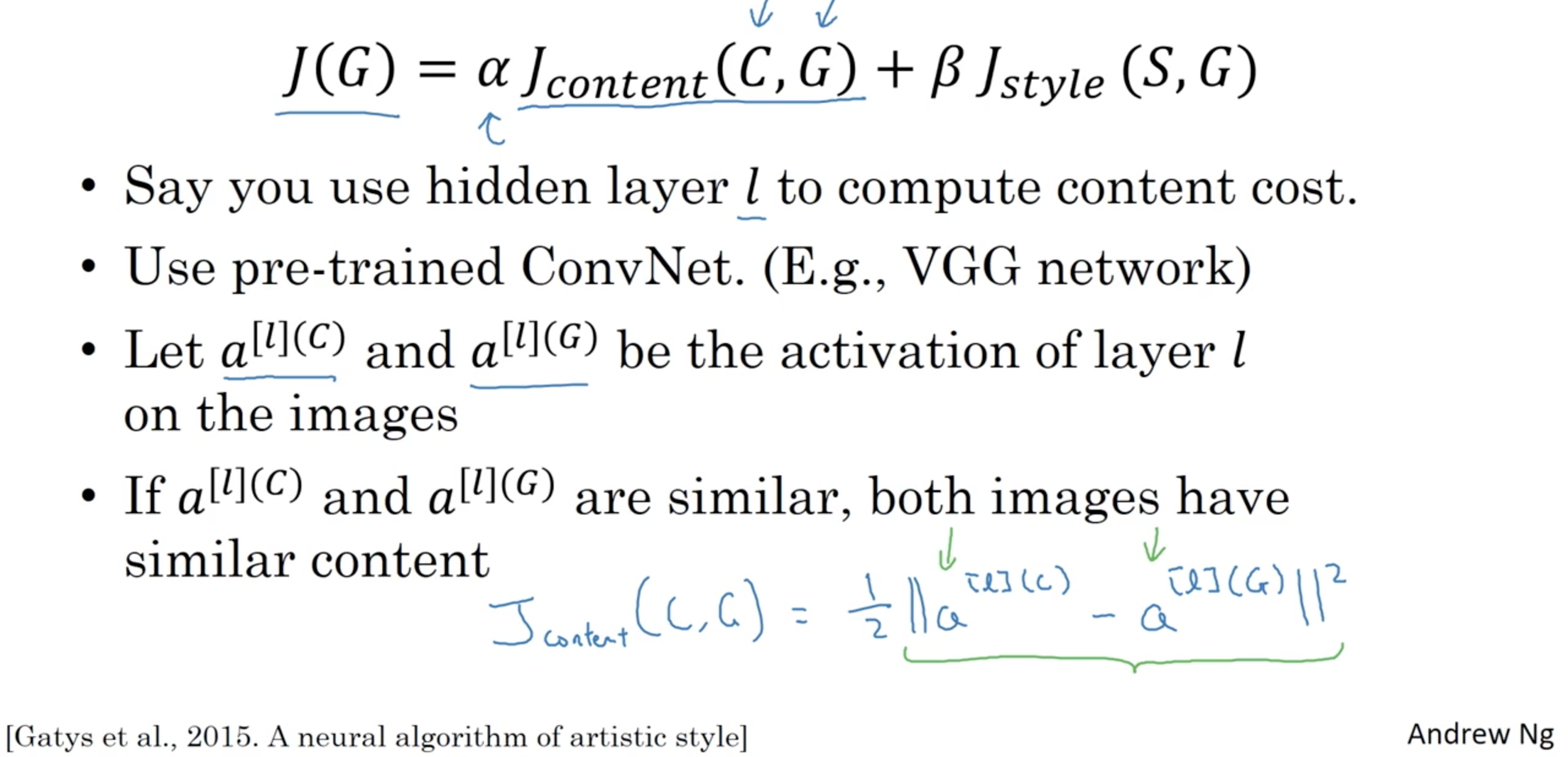
\[J_{\text{content}}(C,G) = \frac{1}{4 \times n_H \times n_W \times n_C}\sum _{ \text{all entries}} (a^{(C)} - a^{(G)})^2\tag{1}\]

Here, $n_H, n_W$ and $n_C$ are the height, width and number of channels of the hidden layer you have chosen

Style cost function

Gram matrix of the “style” image S and that of the “generated” image G. For now, we are using only a single hidden layer $a^{[l]}$, and the corresponding style cost for this layer is defined as:

\[J_{\text{style}}^{[l]}(S,G) = \frac{1}{4 \times {n_C}^2 \times (n_H \times n_W)^2} \sum _{i=1}^{n_C}\sum_{j=1}^{n_C}(G^{(S)}_{ij} - G^{(G)}_{ij})^2\tag{2}\]

where $G^{(S)}$ and $G^{(G)}$ are respectively the Gram matrices of the “style” image and the “generated” image, computed using the hidden layer activations for a particular hidden layer in the network.